8 Model Selection

8.1 Distributional Choice, Model Progression, and Predictive Calibration

This chapter provides the statistical foundation for three claims made implicitly throughout the modelling sequence: that the Zero-Inflated Gamma (ZIG) family is the appropriate distributional choice for this data, that each successive model extension was a genuine improvement rather than an over-fit, and that the final model captures a meaningful share of the predictable structure in Australian rainfall. Each claim is addressed through a distinct formal procedure.

8.2 Predictive Accuracy and Distributional Calibration

Show the code

source(here::here("chapter8", "predictive_accuracy.R"))
render_error_metrics()

Table 8.1: Global predictive error metrics across all observations and locations.

Metric	Error
RMSE	7.567
MAE	2.760

Show the code

render_error_metrics(filter_zeros = TRUE)

Table 8.2: Predictive error metrics restricted to rain-days (positive observations only).

Metric	Error
RMSE	12.263
MAE	5.607

Show the code

plot_ppc(ppc_dat)

Figure 8.1: Posterior Predictive Check. The observed distribution (blue) lies well within the envelope of 50 model-simulated distributions (grey), confirming that the ZIG model replicates the key structural features of the rainfall distribution.

The global error metrics in Table 8.1 provide a compact summary of predictive accuracy across all observations and locations. The mean absolute error (MAE) of 2.760 mm indicates that the model’s point prediction deviates from the recorded value by 2.760 mm on an average observation. The root mean squared error (RMSE) of 7.567 mm is substantially larger, reflecting the asymmetric influence of extreme events: a small number of days on which a major storm was under-predicted exerts a disproportionate upward pull on the squared error average. The gap between MAE and RMSE is therefore informative, confirming that prediction errors are not symmetrically distributed but are concentrated in the right tail.

When the evaluation is restricted to rain-days only (Table 8.2), the RMSE rises to 12.263 mm and the MAE to 5.607 mm, as expected: the zero observations, which are trivially predicted, no longer dilute the error distribution, and the remaining errors reflect the model’s performance on the harder problem of quantifying intensity.

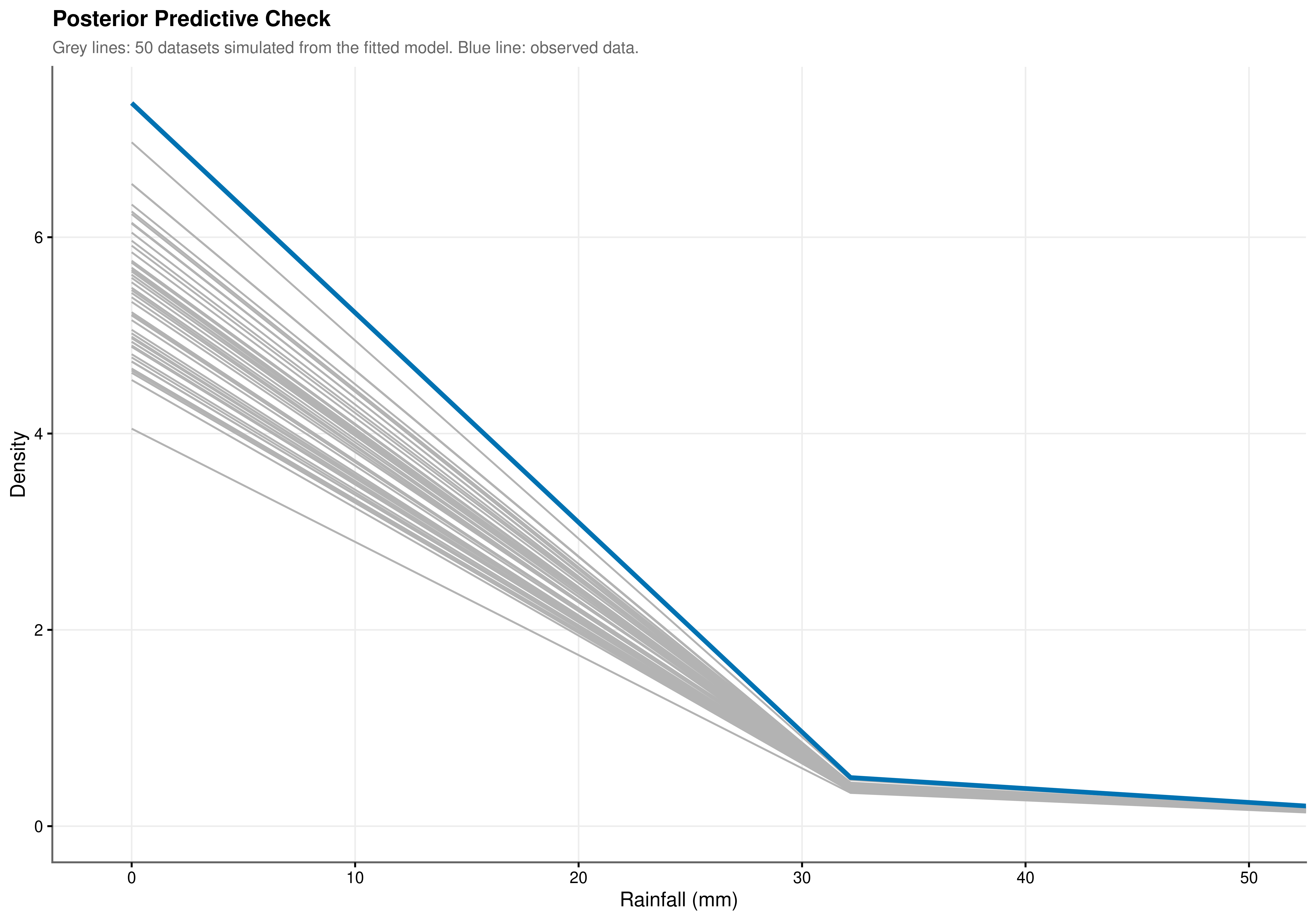
Point error metrics measure accuracy at the conditional mean but cannot assess whether the model is correctly reproducing the entire shape of the rainfall distribution. The posterior predictive check (PPC) in Figure 8.1 addresses this more demanding criterion by simulating 50 complete datasets from the fitted model and overlaying their empirical densities against the observed distribution. Close agreement across the full range of the distribution is apparent. The peak at 0 mm is reproduced accurately, confirming that the zero-inflation component is generating the correct proportion of dry-day predictions conditional on all covariates. The decay rate of the right tail follows the observed data closely, a property that a Gaussian model structurally cannot achieve given its symmetric support. The model is not merely fitting conditional means: it replicates the probabilistic structure of the underlying climate system.

8.3 Justification of the Distributional Family

Show the code

plot_distribution_comparison(check_data)

Figure 8.2: Predictive density comparison across four distributional families. The Gaussian model predicts negative rainfall, a physical impossibility. The lognormal model respects the positive support but cannot represent dry days without a separate zero-inflation mechanism. Both the Tweedie and ZI-Gamma families accommodate zero values and approximate the right tail of the observed distribution.

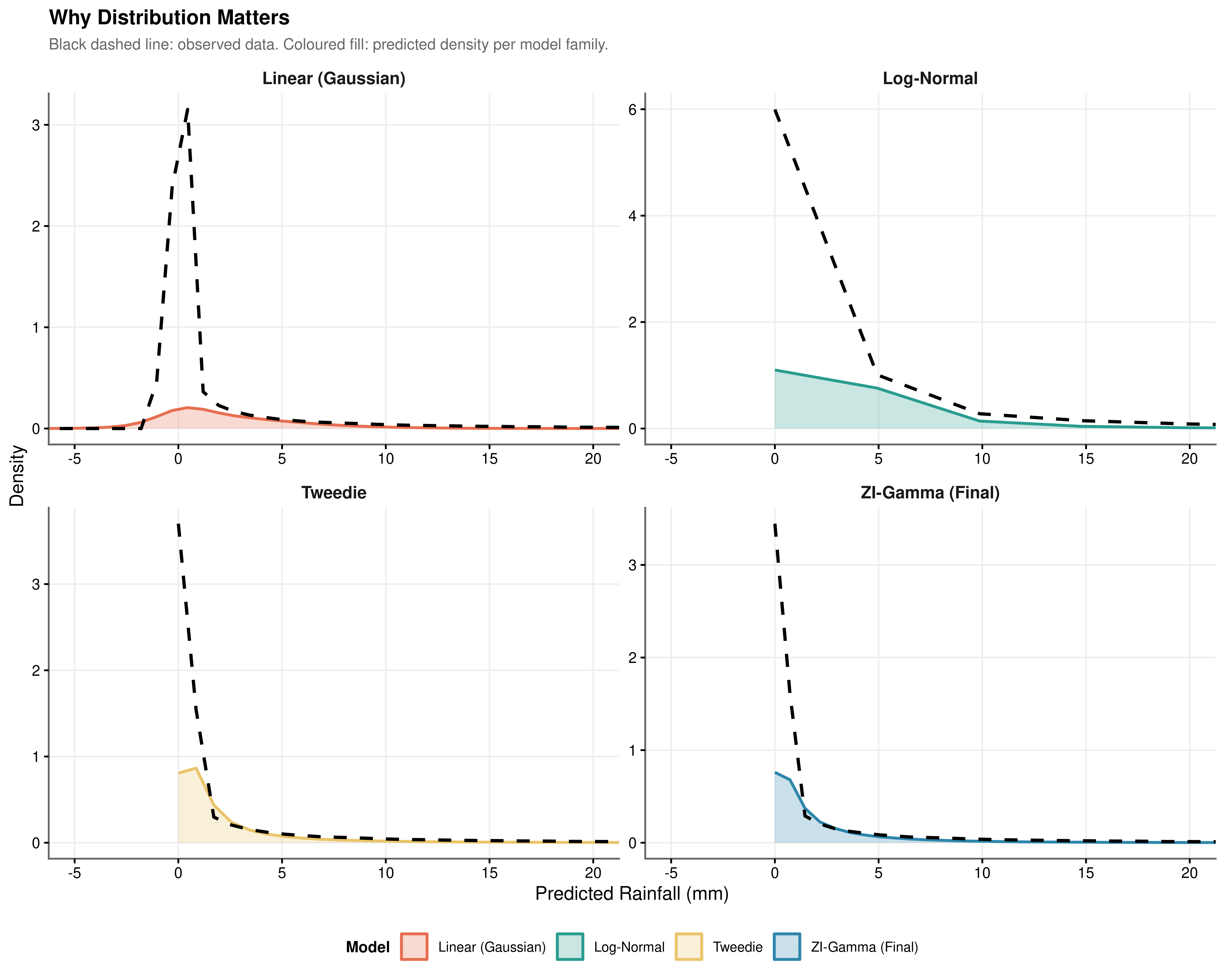
Choosing a distributional family determines the support of the predictions, the variance function, and the structure of the likelihood being optimised. Four families were evaluated against the full predictor set, as shown in Figure 8.2, to isolate the contribution of distributional choice from the contribution of the predictors themselves.

The Gaussian model. A linear mixed model with Gaussian errors generates predictions that extend into negative values. Because the Gaussian distribution has support over the entire real line, the model has no mechanism to prevent this, and negative rainfall is a physical impossibility. The Gaussian assumption also implies a symmetric and constant variance structure, which is incompatible with the heavy right skew and variance-mean dependence documented in Chapter 4. Fitting a Gaussian model to these data produces predictions that are fundamentally inconsistent with the properties of the system being modelled.

The zero-inflated lognormal model. The lognormal hurdle model shares the same two-component structure as the ZIG: a logistic zero-inflation submodel and a lognormal conditional intensity submodel with a log link, fitted via the same predictor sets. It therefore handles the zero mass correctly and does not suffer the structural failure of the Gaussian model. The distinction between the lognormal and Gamma families is instead one of tail behaviour and variance function. The lognormal conditional variance is \(\text{Var}(Y \mid Y > 0) = \mu^2(e^{\sigma^2} - 1)\), where \(\sigma^2\) is the log-scale variance and is treated as a fixed parameter. The Gamma conditional variance is \(\text{Var}(Y \mid Y > 0) = \mu^2 / \phi\), implying a constant coefficient of variation across the range of fitted values. When the coefficient of variation is approximately stable as is consistent with a multiplicative meteorological process in which larger rain events scale proportionally with atmospheric forcing the Gamma variance function is the more appropriate specification. The lognormal, by contrast, imposes a heavier parametric tail structure through \(e^{\sigma^2}\) that is less well-identified when the dispersion parameter must be estimated from a distribution with kurtosis of 181.146. The visual separation between the two families is apparent in Figure 8.2, where the ZIG tail tracks the observed density more closely than the lognormal alternative.

The Tweedie model. The Tweedie distribution with power parameter \(p \in (1, 2)\) is a compound Poisson-Gamma distribution that accommodates zero values alongside a continuous positive component. It respects the zero lower bound and can represent right-skewed positive data. However, it models zeros and positive values through a single unified process governed by a single mean parameter and the power index. The probability of a zero and the expected positive value are both driven by the same linear predictor and cannot respond to different sets of covariates.

The Zero-Inflated Gamma model. The ZIG framework relaxes this constraint explicitly. The zero-inflation and conditional intensity components have separate linear predictors, so predictors of occurrence and predictors of intensity are estimated independently. The EDA provides direct empirical motivation for this separation: the Markov analysis showed that rain_yesterday operates primarily through the hurdle, while the pressure change analysis identified the diurnal pressure signal as more relevant to intensity. These two physical processes do not share the same covariates, and a model that constrains them to do so sacrifices both interpretability and predictive accuracy. The ZIG framework assigns each process its own parameter vector, making it both more flexible and more physically coherent than any of the three alternatives.

8.4 Progressive Model Selection via Pooled \(D_1\) Statistics

Each successive extension was evaluated using the pooled \(D_1\) Wald test (Li, Raghunathan & Rubin 1991), which provides a joint \(F\)-statistic for the parameters added at each step, pooled across multiply imputed datasets via Rubin’s rules. With \(n \approx 142{,}000\) observations, \(D_1\) converges in probability to the \(D_3\) statistic (van Buuren, FIMD), making it the appropriate pooled test for this sample size. The null hypothesis in each case is that the added parameter vector is jointly zero, i.e., that the smaller model is adequate. Delta AIC and delta BIC reported alongside each comparison are heuristic summaries computed from the imputation-averaged log-likelihoods and serve as a secondary consistency check.

Show the code

m0 <- get_model("m0_null")
m1 <- get_model("m1_moisture")

compare_models(m_large = m1, m_small = m0) %>%
  render_comparison_table(names = c("+ Moisture & Pressure", "Null Baseline"))

Table 8.3: Nested Model Comparison: Moisture & Pressure vs. Null Baseline. D1 pooled Wald test across 10 imputed datasets.

Nested Model Comparison: + Moisture & Pressure vs Null Baseline
Test	Parameters tested	F	df1	df2	RIV	p
D1 pooled Wald	Humidity3pm Dewpoint 9am Dewpoint Change Pressure Change	141.806	4	39.8	16.525	<0.001
Note:
† p<0.1 * p<0.05 p<0.01 * p<0.001
delta AIC = -35938.32, delta BIC = -35899.87 (negative favours + Moisture & Pressure; heuristic only). Based on 10 common imputations.
Pooled via Rubin’s rules.

The four moisture and pressure parameters (Humidity3pm, Dewpoint 9am, Dewpoint Change, Pressure Change) are jointly significant at \(F(4,\ 39.8) = 141.806\), \(p < 0.001\), with a relative increase in variance (RIV) of 16.525 reflecting substantial between-imputation variability in the moisture predictors (Table 8.3). The \(\Delta\text{AIC} = -35{,}938.32\) relative to the null represents the largest single gain in the model sequence.

Show the code

m2 <- get_model("m2_temporal")

compare_models(m_large = m2, m_small = m1) %>%
  render_comparison_table(
    names = c("+ Seasonality & Persistence", "Moisture Only")
  )

Table 8.4: Nested Model Comparison: Seasonality & Persistence vs. Moisture Only. D1 pooled Wald test across 10 imputed datasets.

Nested Model Comparison: + Seasonality & Persistence vs Moisture Only
Test	Parameters tested	F	df1	df2	RIV	p
D1 pooled Wald	Day Cos Day Sin ZI: Rain Yesterday (Yes) ZI: Cloud Development	802.158	4	71.3	2.098	<0.001
Note:
† p<0.1 * p<0.05 p<0.01 * p<0.001
delta AIC = -12810.42, delta BIC = -12772.62 (negative favours + Seasonality & Persistence; heuristic only). Based on 10 common imputations.
Pooled via Rubin’s rules.

The seasonal and persistence parameters (Day Cos, Day Sin, ZI: Rain Yesterday, ZI: Cloud Development) yield \(F(4,\ 71.3) = 802.158\), \(p < 0.001\) (Table 8.4). The \(F\)-statistic is the largest in the sequence, driven by the Markov persistence indicator rain_yesterday, whose effect on the zero-inflation submodel is among the strongest individual signals in the model. The \(\Delta\text{AIC} = -12{,}810.42\).

Show the code

m3 <- get_model("m3_history")

compare_models(m_large = m3, m_small = m2) %>%
  render_comparison_table(
    names = c("+ Accumulated History", "Seasonality & Persistence")
  )

Table 8.5: Nested Model Comparison: Accumulated History vs. Seasonality & Persistence. D1 pooled Wald test across 10 imputed datasets.

Nested Model Comparison: + Accumulated History vs Seasonality & Persistence
Test	Parameters tested	F	df1	df2	RIV	p
D1 pooled Wald	Rainfall Ma7 Days Since Rain Humidity Ma7 ZI: Sunshine ZI: Evaporation	275.213	5	177.8	0.902	<0.001
Note:
† p<0.1 * p<0.05 p<0.01 * p<0.001
delta AIC = -4005.81, delta BIC = -3960.45 (negative favours + Accumulated History; heuristic only). Based on 10 common imputations.
Pooled via Rubin’s rules.

The five accumulated history parameters (Rainfall Ma7, Days Since Rain, Humidity Ma7, ZI: Sunshine, ZI: Evaporation) are jointly significant at \(F(5,\ 177.8) = 275.213\), \(p < 0.001\) (Table 8.5). The denominator degrees of freedom of 177.8 are Barnard-Rubin corrected and their relatively large value reflects low between-imputation variability, consistent with the stability of moving-average features across imputed datasets. The \(\Delta\text{AIC} = -4{,}005.81\).

Show the code

m4 <- get_model("m4_energy")

compare_models(m_large = m4, m_small = m3) %>%
  render_comparison_table(
    names = c("+ Thermodynamics & Interaction", "Accumulated History")
  )

Table 8.6: Nested Model Comparison: Thermodynamics & Interaction vs. Accumulated History. D1 pooled Wald test across 10 imputed datasets.

Nested Model Comparison: + Thermodynamics & Interaction vs Accumulated History
Test	Parameters tested	F	df1	df2	RIV	p
D1 pooled Wald	Instability Index Sun Humid Interaction	49.375	2	24.1	4.470	<0.001
Note:
† p<0.1 * p<0.05 p<0.01 * p<0.001
delta AIC = -1066.31, delta BIC = -1028.51 (negative favours + Thermodynamics & Interaction; heuristic only). Based on 10 common imputations.
Pooled via Rubin’s rules.

The thermodynamic and interaction parameters (Instability Index, Sun-Humidity Interaction) yield \(F(2,\ 24.1) = 49.375\), \(p < 0.001\) (Table 8.6). The elevated RIV of 4.470 and the small denominator degrees of freedom indicate that the instability index is sensitive to imputation: the atmospheric instability variable has non-trivial missing data, and its imputed values differ meaningfully across datasets. The point estimate nonetheless clears the significance threshold decisively. The \(\Delta\text{AIC} = -1{,}066.31\).

Show the code

m5 <- get_model("m5_wind")

compare_models(m_large = m5, m_small = m4) %>%
  render_comparison_table(
    names = c("+ Wind Vectors", "Thermodynamics & Interaction")
  )

Table 8.7: Nested Model Comparison: Wind Vectors vs. Thermodynamics & Interaction. D1 pooled Wald test across 10 imputed datasets.

Nested Model Comparison: + Wind Vectors vs Thermodynamics & Interaction
Test	Parameters tested	F	df1	df2	RIV	p
D1 pooled Wald	Gust U EW Gust V NS Wind9am V NS Wind9am U EW	133.422	4	272.8	0.497	<0.001
Note:
† p<0.1 * p<0.05 p<0.01 * p<0.001
delta AIC = -782.35, delta BIC = -752.11 (negative favours + Wind Vectors; heuristic only). Based on 10 common imputations.
Pooled via Rubin’s rules.

The four wind vector parameters (Gust U EW, Gust V NS, Wind9am V NS, Wind9am U EW) yield \(F(4,\ 272.8) = 133.422\), \(p < 0.001\) (Table 8.7). This step produces the smallest absolute AIC reduction in the sequence (\(\Delta\text{AIC} = -782.35\)), yet the \(F\)-statistic is large and the RIV of 0.497 is the smallest in the sequence, indicating that wind direction is well-identified across imputations. The improvement is genuine rather than artefactual.

Show the code

m6 <- get_model("m6_mixed")

compare_models(m_large = m6, m_small = m5) %>%
  render_comparison_table(names = c("+ Random Effects", "Wind Vectors"))

Table 8.8: Nested Model Comparison: Mixed Effects (splines + random intercepts) vs. Wind Vectors. D1 pooled Wald test across 10 imputed datasets.

Nested Model Comparison: + Random Effects vs Wind Vectors
Test	Parameters tested	F	df1	df2	RIV	p
D1 pooled Wald	Dewpoint Change (Spline) Pressure Change (Spline) Evaporation (Spline) Instability Index (Spline, Df=3)1 Instability Index (Spline, Df=3)2 Instability Index (Spline, Df=3)3 Gust U EW (Spline, Df=2)1 Gust U EW (Spline, Df=2)2 Wind9am U EW (Spline, Df=2)1 Wind9am U EW (Spline, Df=2)2	75.283	10	138.9	3.877	<0.001
Note:
† p<0.1 * p<0.05 p<0.01 * p<0.001
delta AIC = -6915.32, delta BIC = -6786.8 (negative favours + Random Effects; heuristic only). Based on 10 common imputations.
Pooled via Rubin’s rules.

The ten spline and random-effect parameters yield \(F(10,\ 138.9) = 75.283\), \(p < 0.001\) (Table 8.8). The \(\Delta\text{AIC} = -6{,}915.32\) is the second largest gain in the sequence, reflecting the substantial explanatory contribution of geographic heterogeneity. The RIV of 3.877 indicates that the non-linear spline terms, particularly the instability index spline and the eastward wind component splines, show meaningful between-imputation variability.

Show the code

source(here::here("chapter8", "model_progression.R"))
model_stats <- build_model_stats()

render_model_summary(model_stats)

Table 8.9: Model selection summary. AIC and BIC are heuristic quantities averaged across imputed datasets. \(\Delta\)AIC is relative to M6, the best model. The Akaike weight of M6 rounds to 1.0 at any practical precision.

Model Selection Summary
Model	AIC	BIC	Δ AIC	Akaike Weight
M6: Mixed Effects	400151.2	400498.9	0.00	1
M5: Wind	407066.5	407285.7	6915.32	0
M4: Energy	407848.8	408037.8	7697.66	0
M3: History	408915.1	409066.3	8763.97	0
M2: Temporal	412920.9	413026.8	12769.78	0
M1: Moisture	425731.4	425799.4	25580.19	0
M0: Null	461669.7	461699.3	61518.51	0

Show the code

plot_aic_trajectory(model_stats)

Figure 8.3: AIC trajectory across the progressive model sequence. Each extension reduces AIC monotonically, confirming that no step introduced net redundancy. The two largest gains correspond to the initial moisture and pressure predictors (M0 to M1) and the final mixed-effects structure (M5 to M6).

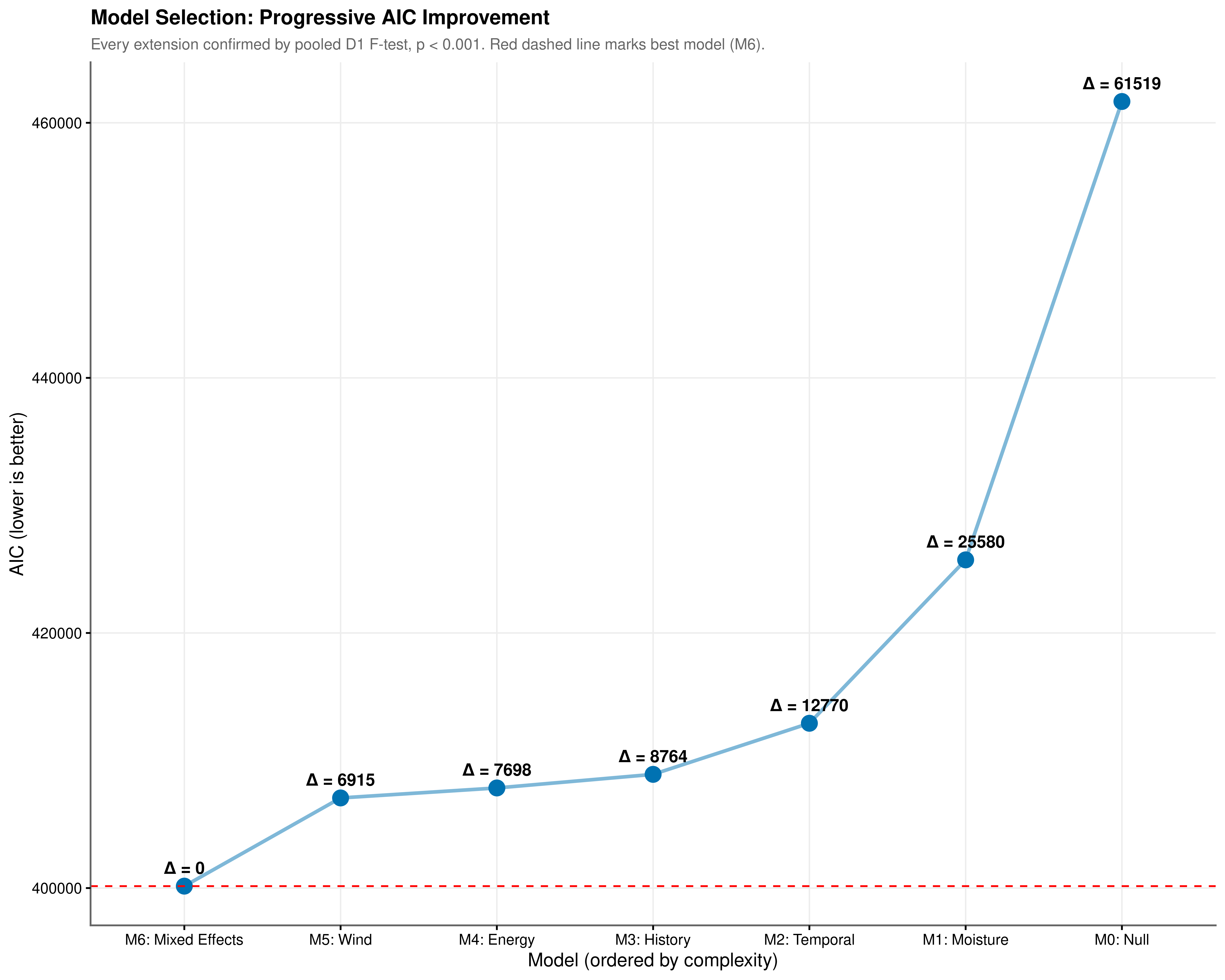
The complete model progression is summarised in Table 8.9 and illustrated in Figure 8.3. AIC quantifies the information lost when a given model approximates the true data-generating process, penalising complexity to discourage over-fitting. A monotonically decreasing AIC sequence is not guaranteed: a predictor block whose likelihood improvement is smaller than its parameter penalty will produce a net AIC increase. The fact that every extension in Figure 8.3 produced a net reduction confirms that each added component captures genuine signal rather than noise.

The pooled \(D_1\) \(F\)-statistics provide the corresponding inferential framework under multiple imputation. For each nested pair, the test evaluates whether the additional parameters are jointly zero, with the \(F\)-statistic and degrees of freedom pooled via Rubin’s rules. The numerator degrees of freedom equal the number of parameters added at each step; the denominator degrees of freedom are Barnard-Rubin corrected and therefore appear as non-integers. All six comparisons reject the null at \(p < 0.001\). Even the step with the smallest absolute AIC gain, the addition of wind vectors from M4 to M5 (\(\Delta\text{AIC} = -782.35\)), yields \(F(4,\ 272.8) = 133.422\), an improvement overwhelmingly inconsistent with chance.

The Akaike weights provide a final calibration. With \(\Delta\text{AIC} = 61{,}518.51\) separating M6 from the null baseline, and a minimum pairwise separation of 782.35 between any two adjacent models, the weight assigned to M6 rounds to 1.0 at any practical decimal precision. There is no information-theoretic basis for preferring any earlier model in the sequence.

8.5 Conclusion

The evidence assembled across this chapter supports three conclusions. First, the ZIG distributional family is the appropriate choice for these data: the Gaussian model produces physically impossible negative predictions, and the Tweedie model, while valid, constrains occurrence and intensity to share the same linear predictor in a manner inconsistent with the distinct physical processes identified in the EDA. Second, every step in the progressive model sequence represents a statistically significant improvement, confirmed by pooled \(D_1\) Wald tests, each rejecting the null at \(p < 0.001\), and by a monotonically decreasing AIC trajectory. The Akaike weight of M6 is effectively 1.0, leaving no information-theoretic basis for preferring any earlier model. Third, the posterior predictive check confirms that the final model reproduces the distributional shape of Australian rainfall across the full support of the response, not only at the conditional mean. The occurrence and intensity components are separately calibrated and jointly coherent with the physical mechanisms motivating the model structure.