7 Model Evaluation
Chapter Context. A model that fits training data well is not necessarily a model that is correct. This chapter subjects the final mixed-effects ZIG model (M6) to four distinct validation procedures, each targeting a different potential failure mode: poor discriminative ability in the occurrence submodel, spatially inappropriate parameter homogeneity, distributional misspecification in the residuals, and unabsorbed temporal autocorrelation. Together, these tests form a coherent audit of the model’s assumptions and capabilities.
7.1 Classification Performance of the Occurrence Submodel
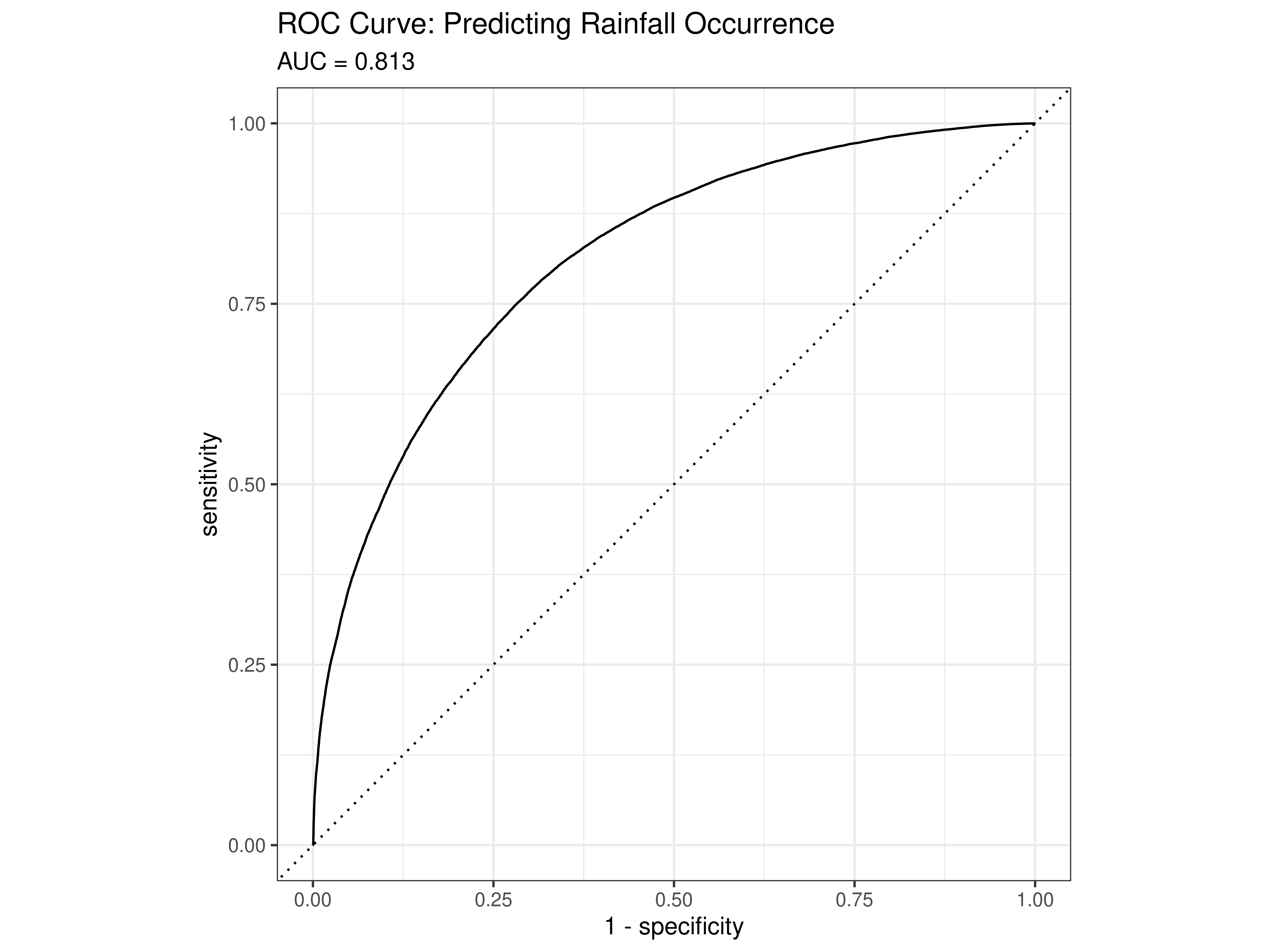
Although the ZIG model is primarily a framework for predicting rainfall amount, its zero-inflation component constitutes a binary classifier at each observation: it assigns a probability that the day is structurally dry. Evaluating this component as a classifier allows direct assessment of how well the model separates the two fundamentally different weather states identified in Chapter 4.
Discriminative ability. The area under the ROC curve is 0.813 (Figure 7.1), meaning that in 81.3% of randomly drawn pairs consisting of one genuinely dry day and one genuinely wet day, the model correctly assigns the higher dryness probability to the dry day. This threshold-free measure of separation indicates strong discriminative performance for a meteorological classification problem of this complexity.
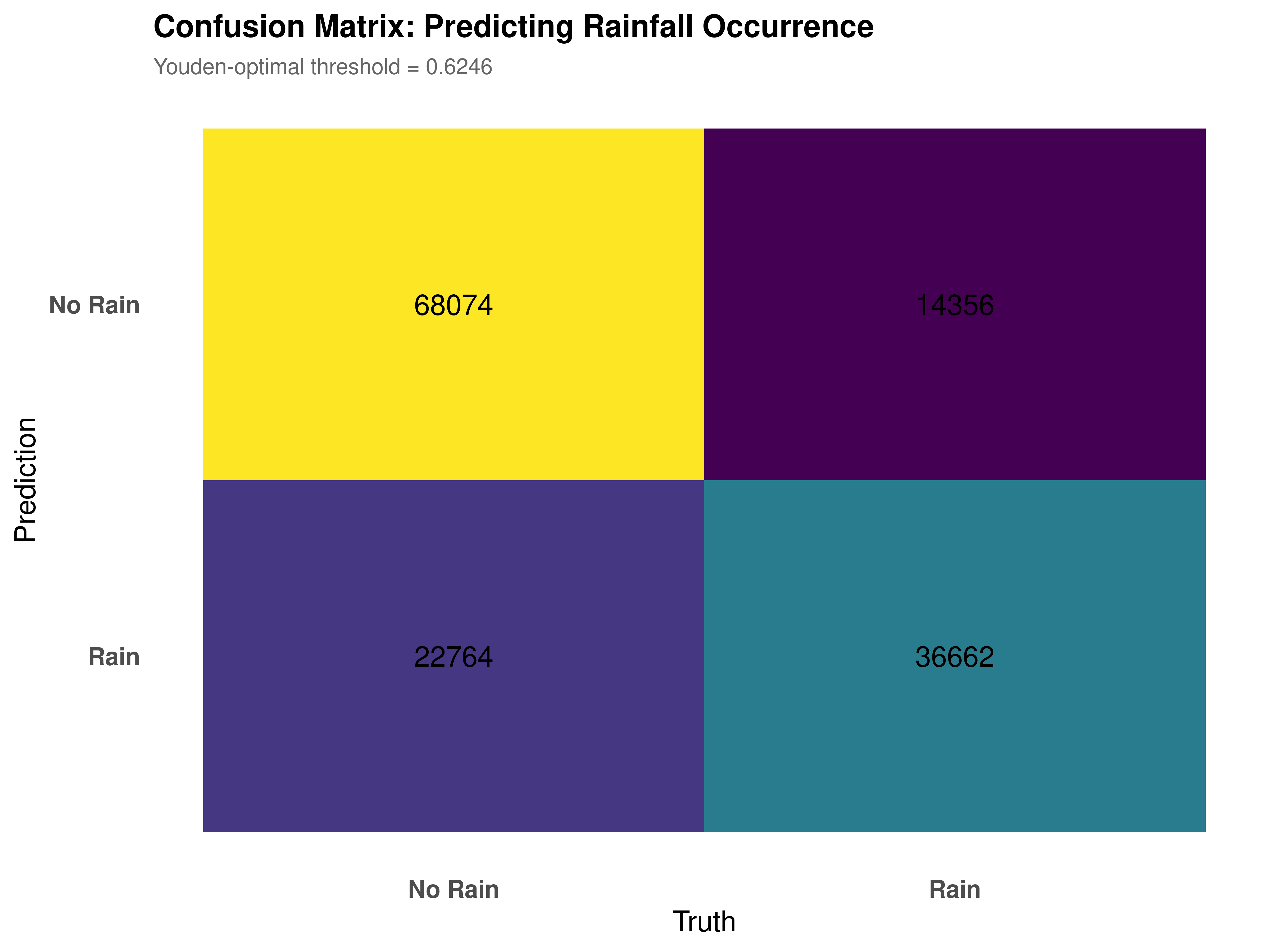
Threshold selection. The raw zero-inflation probability must be converted to a binary prediction through a threshold. Youden’s J statistic, which maximises the sum of sensitivity and specificity simultaneously, selects an optimal threshold of 0.6246. This is notably higher than the naive 0.5 default because dry days constitute 64% of the sample: the model’s calibrated prior assigns moderate dryness probability to many observations by default, and a higher threshold requires more decisive evidence before predicting “No Rain.”
Confusion matrix. At this threshold, the model produces 68,074 correct dry-day predictions (true negatives), 36,662 correct rain predictions (true positives), 22,764 false alarms (predicted dry, actually wet), and 14,356 missed rain events (predicted wet, actually dry) (Figure 7.2). The model generates false alarms at roughly twice the rate at which it misses rain events. In a meteorological context this asymmetry is operationally desirable: the consequence of carrying an umbrella on a dry day is trivial compared to the consequence of being unprepared for a significant rainfall event.
The Brier Score is 0.1654 and the Brier Skill Score is 0.2819, indicating meaningful improvement over a climatological reference forecast.
7.2 Spatial Heterogeneity and Random Effects
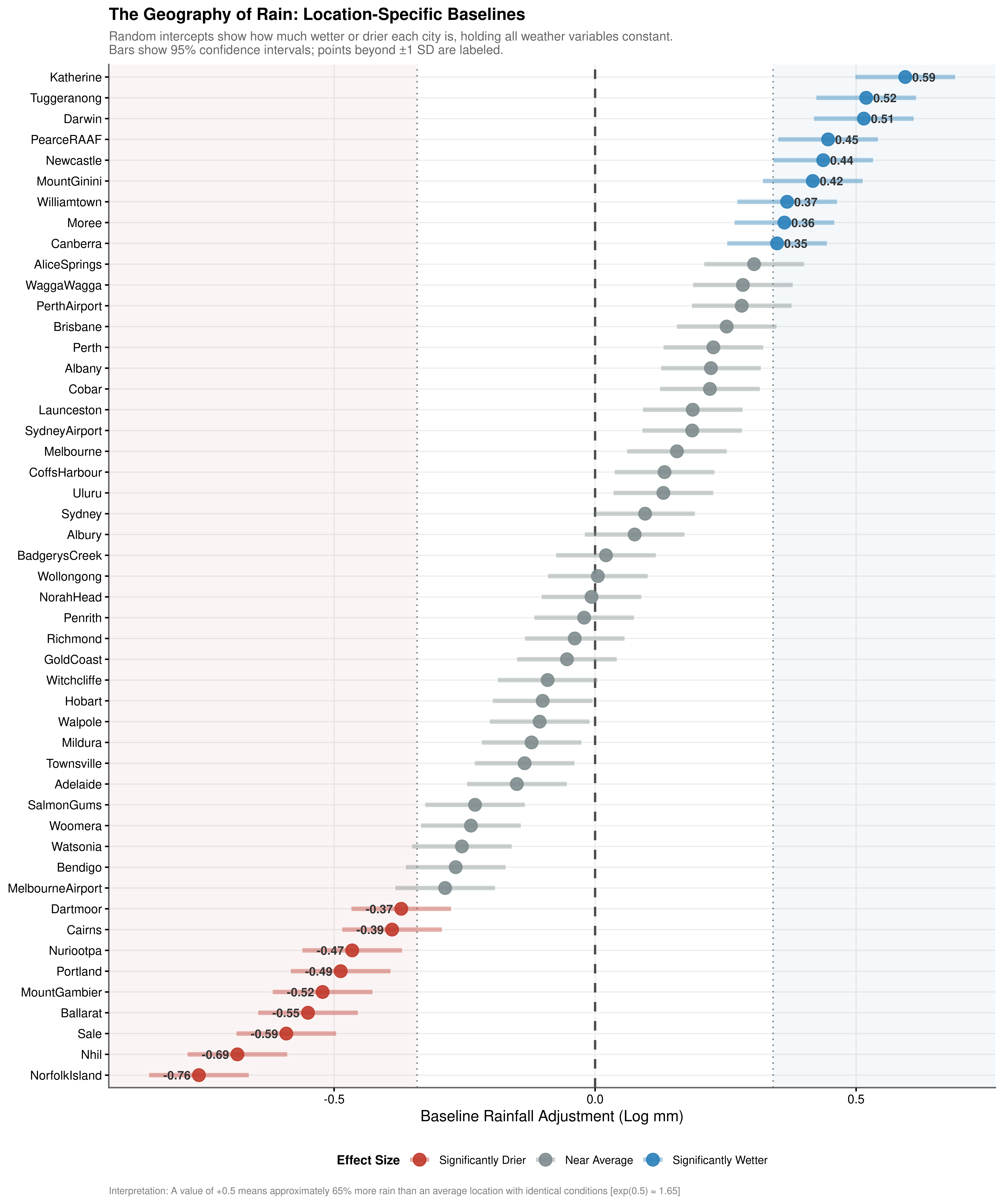
The random intercepts represent the location-specific baseline deviations in rainfall intensity after removing the contribution of all dynamic weather variables humidity, pressure, wind, seasonality, and persistence (Figure 7.3). What remains is the component of rainfall attributable to geographic and climatic factors that do not vary day-to-day: proximity to moisture sources, orographic effects, predominant circulation patterns, and regional climate regime.
The wetter locations. Katherine (\(\hat{b} = 0.59\), \(e^{0.59} \approx 1.80\)) and Tuggeranong (\(\hat{b} = 0.52\), \(e^{0.52} \approx 1.68\)) sit at the high end of the distribution, producing roughly 68% and 80% more rainfall respectively than a hypothetical average Australian location experiencing identical instantaneous weather conditions. Katherine’s elevated baseline is geographically coherent: it sits in the tropical Top End of the Northern Territory, where monsoonal systems deliver sustained and intense rainfall with no structural analogue in the temperate south. Tuggeranong is located in the Australian Capital Territory near Canberra, where its elevated baseline reflects orographic enhancement from the surrounding Brindabella Ranges and exposure to moisture-bearing easterly flows that the dynamic predictors do not fully represent on a day-to-day basis.
The drier locations. Nhil (\(\hat{b} = -0.69\), \(e^{-0.69} \approx 0.50\)) and Norfolk Island (\(\hat{b} = -0.76\), \(e^{-0.76} \approx 0.47\)) show the strongest negative adjustments. Nhil produces roughly half the rainfall of an average location given identical weather conditions, reflecting its position in the semi-arid Wimmera region of inland Victoria where even moisture-laden air masses tend to deliver less precipitation than they would at the coast.
Justification for the mixed-effects structure. The magnitude and geographic coherence of these deviations confirm the necessity of the random effects component. A pooled fixed-effects model would suppress this spatial variation, producing coefficients that systematically over-predict rainfall in arid interior stations and under-predict it in high-rainfall locations. The mixed-effects structure allows the global physical relationships humidity drives intensity, southerly winds bring moisture to remain stable as fixed effects while accommodating the geographically variable baseline against which they operate.
7.3 Residual Diagnostics via DHARMa Simulation
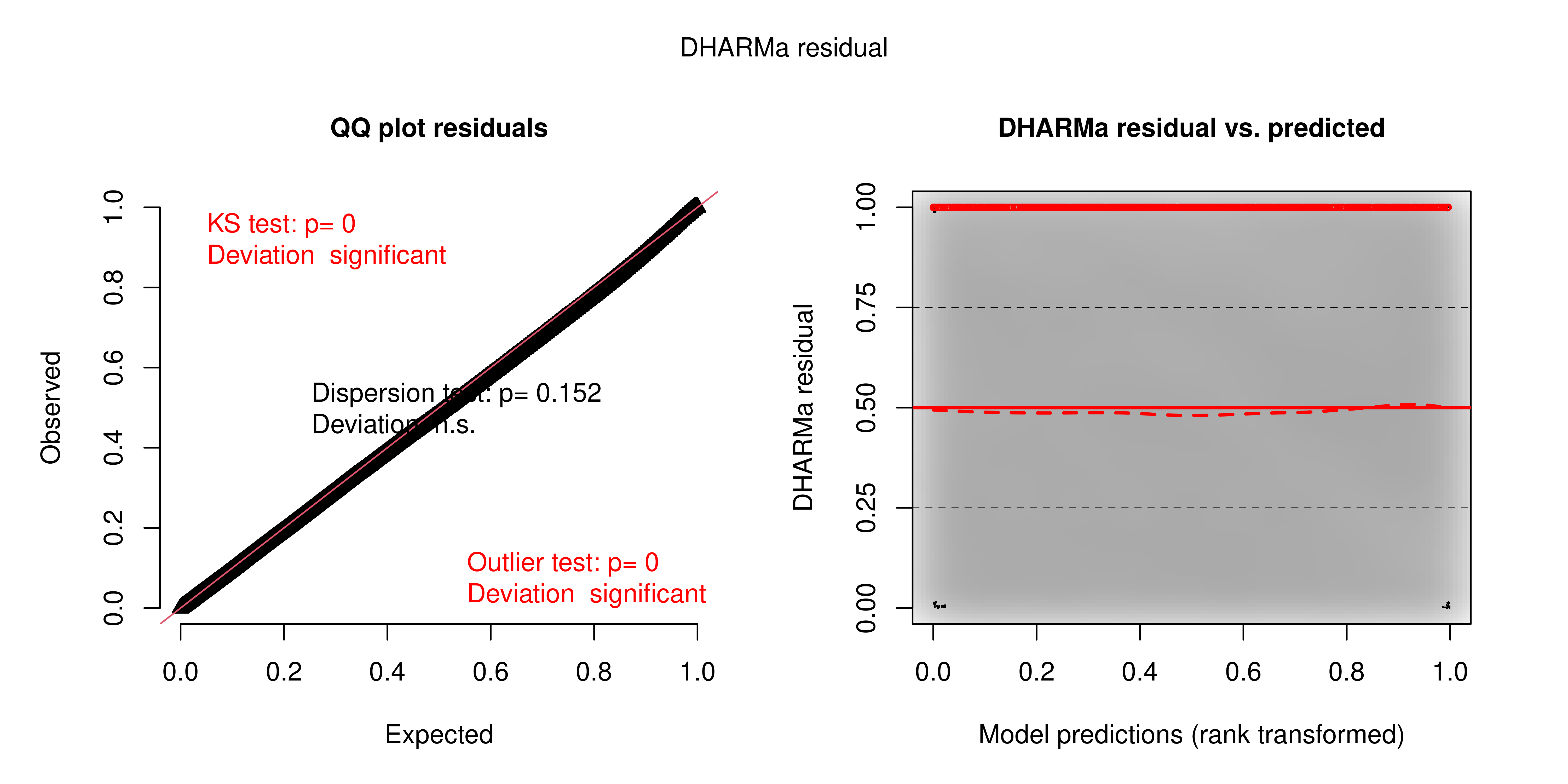
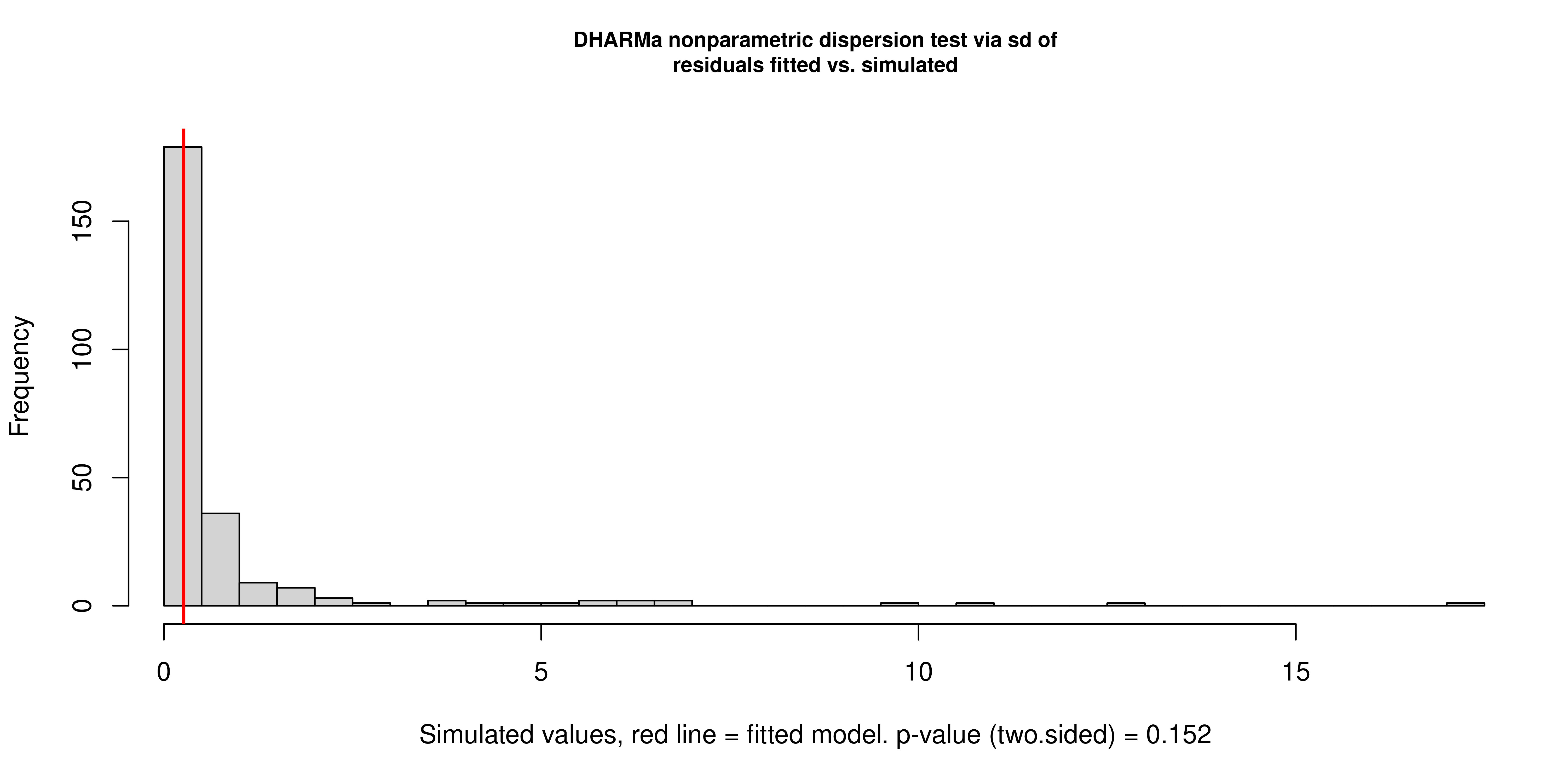
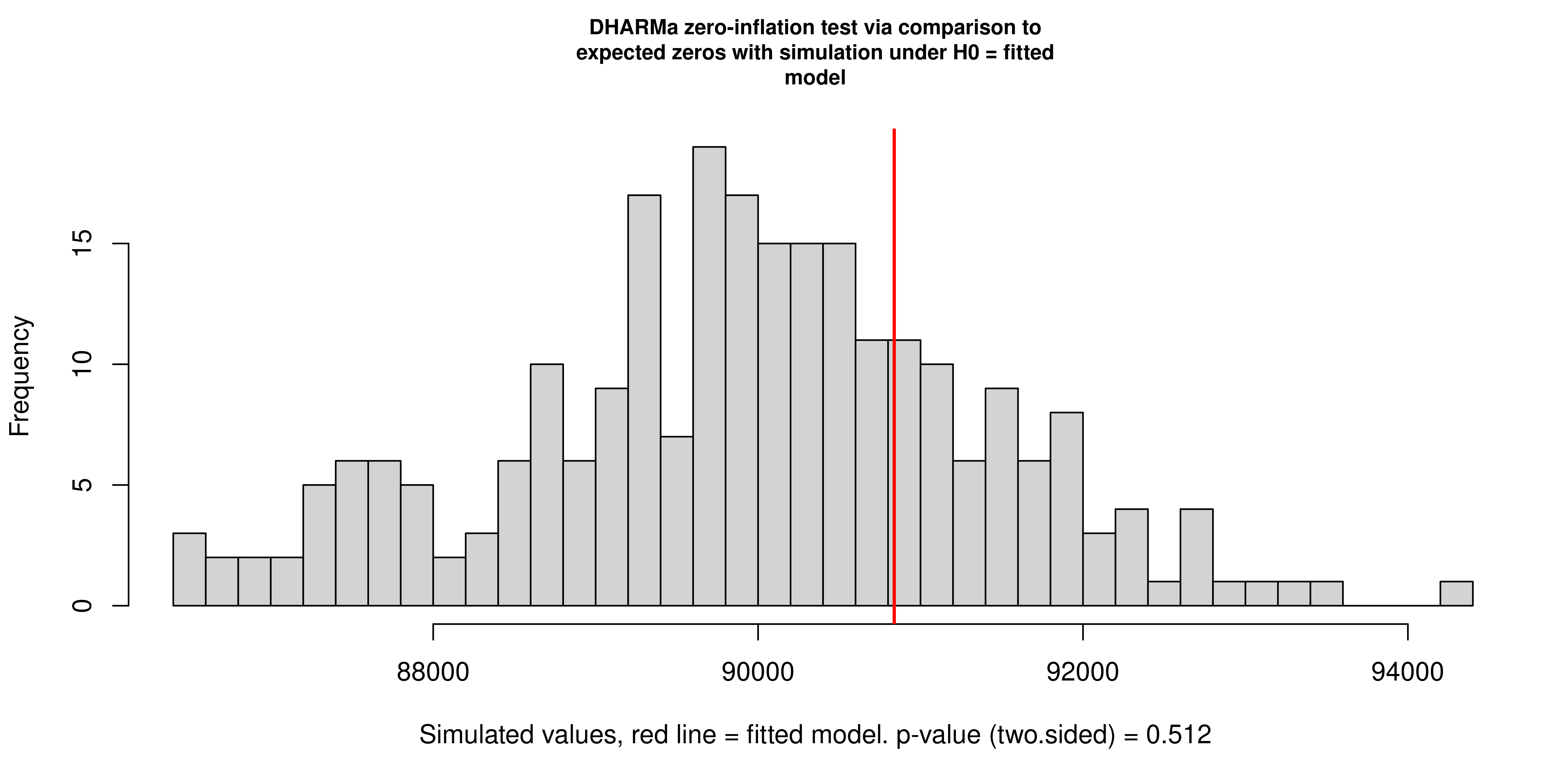
Standard residual diagnostics are not directly applicable to Zero-Inflated Gamma models: the mixture of a point mass at zero and a continuous positive distribution means that conventional Pearson or deviance residuals do not have a tractable reference distribution. DHARMa addresses this by generating a large number of simulated datasets from the fitted model and computing, for each observation, where the actual value falls in the empirical distribution of simulated values. Under a correctly specified model, these scaled residuals follow a uniform distribution on \([0, 1]\) regardless of the model family. Deviations from uniformity indicate misspecification.
Q-Q plot. The empirical quantiles of the scaled residuals align closely with the theoretical diagonal across the full range of the distribution. The Kolmogorov-Smirnov test registers \(p < 0.05\), but this outcome is expected and should not be interpreted as evidence of meaningful misfit: with \(N > 140{,}000\) observations, the test has sufficient power to detect deviations of negligible practical magnitude. The visual alignment of the Q-Q plot, the appropriate diagnostic at this sample size shows no systematic departure from the uniform reference.
Residuals versus predicted. The three quantile lines (25th, 50th, and 75th percentiles of the scaled residuals at each fitted value) are horizontal and evenly spaced across the range of predictions. This indicates the absence of systematic non-linearity and the absence of heteroscedasticity. The model performs with equivalent fidelity across the full range of rainfall intensities, from light drizzle to extreme events.
7.4 Temporal Autocorrelation in Residuals
The most consequential assumption to verify in a time-series regression is whether the residuals are serially independent. If the model has failed to capture all temporal structure in the data, residuals from consecutive days will be correlated, violating the assumption of independent errors and producing standard errors that are too small, confidence intervals that are too narrow, and significance tests that are anti-conservative.
This risk is particularly salient here. The raw data shows strong temporal autocorrelation: yesterday’s rain state, the weekly wetness trend, and the dry spell dynamics all create day-to-day dependencies that, if unmodelled, would produce heavily autocorrelated residuals. The model addresses this through multiple temporal mechanisms: the Markov persistence feature rain_yesterday, the 7-day moving average features, the natural spline of days_since_rain, and the cyclical seasonal encoding.
Results across all locations. The Durbin-Watson test was applied to residuals from all 49 stations and results are reported in Table 7.1, sorted by p-value. The theoretical value under perfect serial independence is 2.0; values below 2 indicate positive autocorrelation and values above 2 indicate negative autocorrelation. The distribution of test statistics across stations reveals a consistent pattern: nearly all values fall in the range 1.81 to 2.25, indicating that the residuals are close to independence everywhere, though the degree of remaining structure varies by location.
Stations with the least residual autocorrelation. Woomera (DW = 2.0021, \(p\) = 0.955), Brisbane (DW = 2.0083, \(p\) = 0.816), Perth (DW = 2.0109, \(p\) = 0.759), and Alice Springs (DW = 2.0139, \(p\) = 0.703) show statistics that are essentially indistinguishable from the ideal value of 2.0. These are predominantly arid or subtropical interior locations where rainfall is episodic and driven by synoptic-scale events well-captured by the dynamic predictors. The temporal engineering has absorbed virtually all day-to-day dependence for these stations.
Stations with the strongest residual autocorrelation. Ballarat (DW = 2.2527, \(p\) < 0.001), Watsonia (DW = 2.2000, \(p\) < 0.001), Cairns (DW = 1.8149, \(p\) < 0.001), and Melbourne Airport (DW = 2.1613, \(p\) < 0.001) sit at the extremes of the distribution. Ballarat and Watsonia, both in the Victorian highlands, show mild negative autocorrelation (DW > 2), suggesting a slight tendency for above-average residuals to follow below-average ones a pattern consistent with orographic rainfall variability that the current predictor set does not fully resolve. Cairns shows mild positive autocorrelation (DW < 2), consistent with multi-day monsoon persistence in tropical North Queensland that the 7-day moving average partially but not entirely captures.
Overall assessment. The majority of stations cluster near DW = 2.0 with \(p\)-values well above conventional thresholds, indicating that the temporal feature engineering was effective across the network as a whole. The residual autocorrelation at a handful of high-rainfall or orographically complex locations is modest in magnitude and does not undermine the validity of the model’s inference; it does, however, identify locations where richer temporal or topographic predictors could yield further improvement.
7.5 Summary of Validation Results
The four validation procedures converge on a consistent picture of a well-specified model. The occurrence submodel achieves strong discriminative separation between dry and wet days, with a conservative error asymmetry appropriate for meteorological risk communication. The random effects structure captures geographically coherent spatial heterogeneity that a pooled model would suppress, with tropical and orographically exposed locations producing substantially more rainfall than the national average and semi-arid interior locations substantially less. The DHARMa diagnostics show close alignment to the uniform reference distribution with no systematic non-linearity or heteroscedasticity across the range of fitted values. The Durbin-Watson tests across all 49 stations confirm that the model’s persistence and dry spell features have successfully eliminated serial dependence from the residuals at the large majority of locations, with modest residual autocorrelation confined to a small number of orographically complex or strongly monsoonal sites. Together, these results support the conclusion that M6 is both statistically valid and physically well-grounded.