4 Exploratory Data Analysis – Australian Rainfall Dynamics

4.1 Data Quality Summary

The missingness diagnostics and imputation pipeline are documented in full in Chapter 2. Briefly: sunshine and evaporation are missing in 47.7% and 42.5% of records respectively, their missingness is station-conditional rather than outcome-conditional, and both are recovered via predictive mean matching across ten imputed datasets. The imputed dataset df_final is used throughout the remainder of this chapter; df_clean is used only in this opening section to avoid circularity between imputed features and the response distribution.

Modelling implication. Discarding sunshine and evaporation would sacrifice two of the strongest predictors of rainfall occurrence (see Section 4.3); listwise deletion would eliminate nearly half the dataset and introduce geographic bias toward well-instrumented stations.

Show the code

total_na <- sum(is.na(df_clean))
print(paste("Total missing values:", total_na))

#> [1] "Total missing values: 314146"

Show the code

missing_val(df_clean)

4.2 Distributional Properties of the Target Variable

Understanding the marginal distribution of the response variable is a prerequisite for selecting an appropriate model family. A Gaussian assumption carries substantive claims about the data-generating process that can be directly tested.

Show the code

source(here::here("chapter4", "target.R"))
render_descriptive_stats()

Table 4.1: Descriptive statistics of daily rainfall (mm).

Descriptive Statistics: Daily Rainfall (mm)
Statistic	Value
n	1.42e+05
mean	2.361
median	0
sd	8.478
min	0
max	371
q25	0
q75	0.8
iqr	0.8
n_zeros	9.11e+04
pct_zeros	64.051
n_large	151
pct_large	0.106
skewness	9.836
kurtosis	181.146

Show the code

render_prevalence_table()

Table 4.2: Prevalence of zero-inflation (dry days) in the rainfall record.

Prevalence of Zero-Inflation (Dry Days)
Total Days	Dry Days (0 mm)	Rainy Days (>0 mm)	Zero Inflation (%)
142199	91080	51119	64.05108

The descriptive statistics reveal a distribution fundamentally incompatible with Gaussian modelling assumptions.

Zero-inflation. 64.05% of the 142,199 recorded observations are dry days (rainfall = 0 mm). The median is zero. The data-generating mechanism produces two qualitatively different outcomes: no rain at all versus some positive amount. Any model treating the response as a single continuous variable will be forced to place probability mass on negative values and will systematically misestimate the probability of the zero outcome.

Heavy tails. Among non-zero observations, the distribution is severely right-skewed (skewness = 9.836). The standard deviation (8.478 mm) is nearly four times the mean (2.361 mm). Kurtosis of 181.146 relative to 3 for a normal distribution confirms that extreme events occur far more frequently than a Gaussian model would predict. The maximum recorded value is 371 mm, and 151 events exceed 100 mm.

Modelling implication. The conjunction of zero-inflation and extreme positive skew means a single-component model is insufficient. The data implicitly poses two separate questions: does rain occur, and given that it does, how much falls? This motivates the Zero-Inflated Gamma framework adopted in subsequent analysis.

4.3 Bivariate Correlation Structure

Because rainfall is heavily skewed and the relationships are unlikely to be linear, Spearman rank correlation is used throughout, a non-parametric measure that captures monotonic association without requiring linearity or normality.

Show the code

source(here::here("chapter4", "correlation.R"))
render_correlation_table()

Table 4.3: Spearman rank correlation with rainfall, ranked by absolute strength.

Spearman Correlation with Rainfall (Ranked by Strength)
Predictor	Correlation (r)	Strength
humidity9am	0.440	Moderate
humidity3pm	0.440	Moderate
sunshine	-0.400	Moderate
cloud9am	0.370	Moderate
cloud3pm	0.320	Moderate
evaporation	-0.310	Moderate
temp3pm	-0.310	Moderate
max_temp	-0.300	Moderate
pressure9am	-0.150	Small
temp9am	-0.150	Small
wind_gust_speed	0.130	Small
wind_speed9am	0.083	Negligible
wind_speed3pm	0.068	Negligible
pressure3pm	-0.063	Negligible
min_temp	0.022	Negligible

Show the code

plot_correlation_matrix()

Figure 4.1: Spearman correlation matrix of meteorological features. Red indicates negative correlation; blue indicates positive correlation. Coefficients are shown only for pairs where |r| > 0.3 to reduce visual noise.

Show the code

run_cocor_test()
#> $pearson1898
#> 
#>  Pearson and Filon's z (1898)
#> 
#> data:  
#> 
#> alternative hypothesis: true difference in correlations is not equal to 0
#> sample estimates:
#>   r.jk.rho   r.jh.rho       r.kh 
#>  0.4436352 -0.4013063 -0.6206376 
#> 
#> 
#> $hotelling1940
#> 
#>  Hotelling's t (1940)
#> 
#> data:  
#> 
#> alternative hypothesis: true difference in correlations is not equal to 0
#> sample estimates:
#>   r.jk.rho   r.jh.rho       r.kh 
#>  0.4436352 -0.4013063 -0.6206376 
#> 
#> 
#> $williams1959
#> 
#>  Williams' t (1959)
#> 
#> data:  
#> 
#> alternative hypothesis: true difference in correlations is not equal to 0
#> sample estimates:
#>   r.jk.rho   r.jh.rho       r.kh 
#>  0.4436352 -0.4013063 -0.6206376 
#> 
#> 
#> $hendrickson1970
#> 
#>  Hendrickson, Stanley, and Hills' (1970) modification of Williams' t
#>  (1959)
#> 
#> data:  
#> 
#> alternative hypothesis: true difference in correlations is not equal to 0
#> sample estimates:
#>   r.jk.rho   r.jh.rho       r.kh 
#>  0.4436352 -0.4013063 -0.6206376 
#> 
#> 
#> $olkin1967
#> 
#>  Olkin's z (1967)
#> 
#> data:  
#> 
#> alternative hypothesis: true difference in correlations is not equal to 0
#> sample estimates:
#>   r.jk.rho   r.jh.rho       r.kh 
#>  0.4436352 -0.4013063 -0.6206376 
#> 
#> 
#> $dunn1969
#> 
#>  Dunn and Clark's z (1969)
#> 
#> data:  
#> 
#> alternative hypothesis: true difference in correlations is not equal to 0
#> sample estimates:
#>   r.jk.rho   r.jh.rho       r.kh 
#>  0.4436352 -0.4013063 -0.6206376 
#> 
#> 
#> $steiger1980
#> 
#>  Steiger's (1980) modification of Dunn and Clark's z (1969) using
#>  average correlations
#> 
#> data:  
#> z = 188.91, p-value < 2.2e-16
#> alternative hypothesis: true difference in correlations is not equal to 0
#> sample estimates:
#>   r.jk.rho   r.jh.rho       r.kh 
#>  0.4436352 -0.4013063 -0.6206376 
#> 
#> 
#> $meng1992
#> 
#>  Meng, Rosenthal, and Rubin's z (1992)
#> 
#> data:  
#> 
#> alternative hypothesis: true difference in correlations is not equal to 0
#> sample estimates:
#>   r.jk.rho   r.jh.rho       r.kh 
#>  0.4436352 -0.4013063 -0.6206376 
#> 
#> 
#> $hittner2003
#> 
#>  Hittner, May, and Silver's (2003) modification of Dunn and Clark's z
#>  (1969) using a backtransformed average Fisher's (1921) Z procedure
#> 
#> data:  
#> 
#> alternative hypothesis: true difference in correlations is not equal to 0
#> sample estimates:
#>   r.jk.rho   r.jh.rho       r.kh 
#>  0.4436352 -0.4013063 -0.6206376 
#> 
#> 
#> $zou2007
#> 
#>  Zou's (2007) confidence interval
#> 
#> data:  
#> 
#> alternative hypothesis: true difference in correlations is not equal to 0
#> sample estimates:
#>   r.jk.rho   r.jh.rho       r.kh 
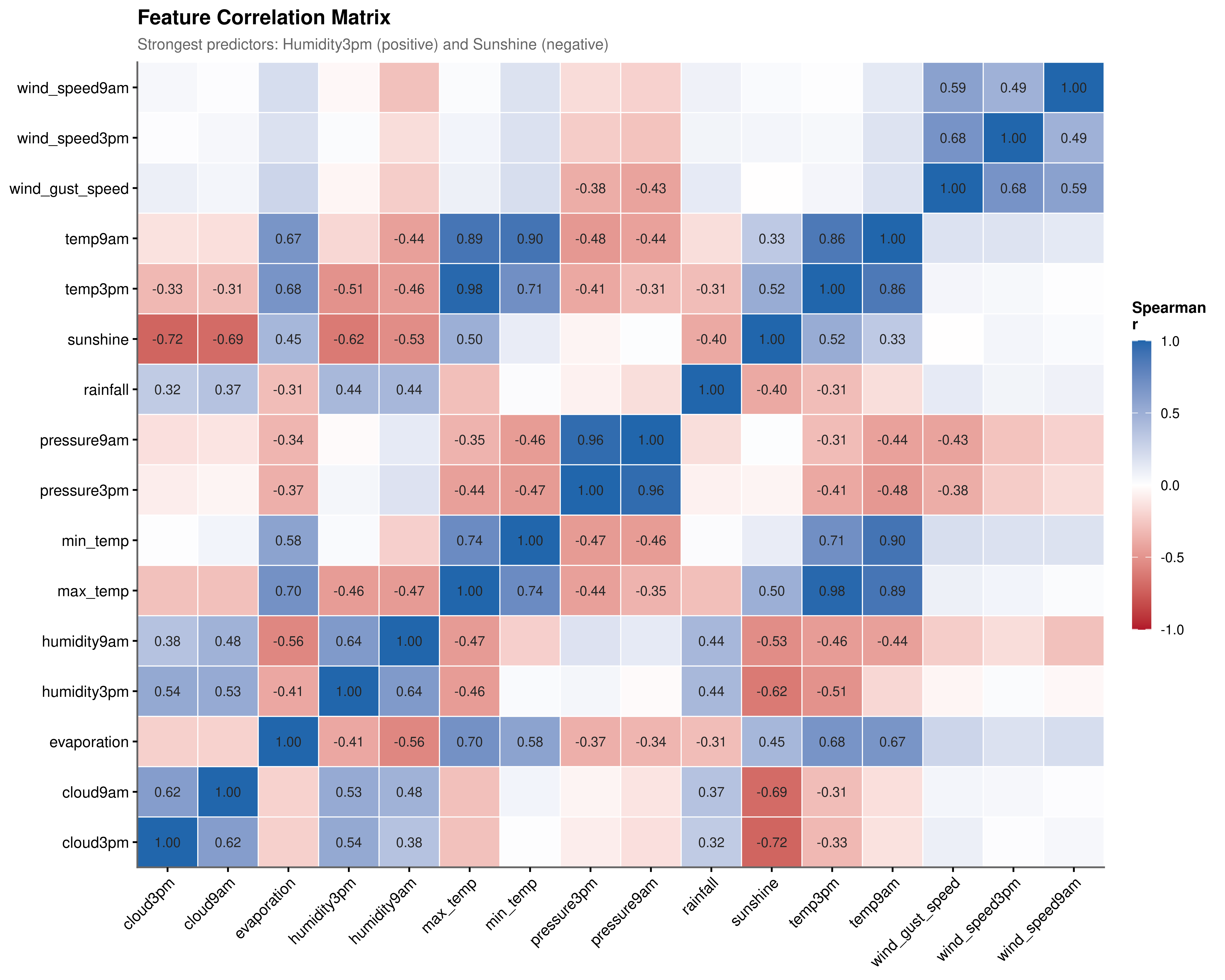
#>  0.4436352 -0.4013063 -0.6206376

Moisture indicators (positive association). Humidity3pm (\(r = 0.44\)) and cloud cover (\(r \approx 0.37\)) show the strongest positive associations. High afternoon humidity indicates that moisture has accumulated in the lower atmosphere over the course of the day. Cloud cover is both a physical precondition for rain and a consequence of the same atmospheric dynamics that produce it.

Radiation and evaporation indicators (negative association). Sunshine (\(r = -0.40\)) and evaporation (\(r = -0.31\)) show the strongest negative associations. Long sunshine hours proxy clear-sky, high-pressure conditions. High evaporation signals warm, dry, low-humidity surface conditions.

Multicollinearity. The correlation heatmap (Figure 4.1) reveals substantial redundancy among predictors. pressure9am and pressure3pm share \(r = 0.96\), and the two temperature readings are similarly collinear. This directly motivates VIF-based feature selection in the feature engineering chapter.

Statistical validation. Steiger’s Z-test comparing the two strongest opposing predictors yields \(z \approx 188.9\), \(p < 2.2 \times 10^{-16}\). With \(N > 140{,}000\), the p-value alone is uninformative; the Z-statistic magnitude confirms that the differential predictive strength is not a sampling artefact. Humidity and sunshine represent genuinely distinct physical forces operating in opposing directions.

4.4 Temporal Structure of Rainfall

4.4.1 Weekly and Seasonal Frequency

Show the code

source(here::here("chapter4", "temporal.R"))
render_weekly_frequency_table()

Table 4.4: Frequency of rainfall days by day of the week.

Frequency of Rainfall Days by Day of the Week
Day	Count (n)	Percentage
Tue	7508	14.7%
Mon	7480	14.6%
Fri	7378	14.4%
Wed	7342	14.4%
Thu	7314	14.3%
Sat	7057	13.8%
Sun	7040	13.8%

Show the code

render_monthly_frequency_table()

Table 4.5: Frequency of rainfall days by month.

Frequency of Rainfall Days by Month
Month	Count (n)	Percentage
6	5448	10.7%
7	5250	10.3%
5	4937	9.7%
8	4704	9.2%
3	4444	8.7%
9	4234	8.3%
4	4001	7.8%
10	3770	7.4%
11	3760	7.4%
1	3702	7.2%
12	3562	7.0%
2	3307	6.5%

Show the code

render_month_day_crosstab()

Table 4.6: Cross-tabulation of rainfall frequency by month and day of week.

Cross-tabulation of Rainfall Frequency: Month vs. Day
month	Sun	Mon	Tue	Wed	Thu	Fri	Sat	Total
1	536	570	514	482	493	567	540	3702
2	480	530	469	466	443	471	448	3307
3	636	645	639	592	662	644	626	4444
4	578	597	566	604	579	515	562	4001
5	710	722	765	714	678	681	667	4937
6	766	801	804	797	760	753	767	5448
7	694	717	728	796	773	818	724	5250
8	612	702	694	679	689	687	641	4704
9	516	571	616	639	648	659	585	4234
10	507	606	579	550	517	456	555	3770
11	556	526	554	480	538	575	531	3760
12	449	493	580	543	534	552	411	3562
Total	7040	7480	7508	7342	7314	7378	7057	51119

Weekly cycle. The distribution of wet days across days of the week is approximately uniform, ranging from 13.8% to 14.7% (Table 4.4). Atmospheric processes operate independently of the social calendar, and the slight variation is consistent with sampling noise. Day carries little predictive information.

Annual cycle. June (10.7%) and July (10.3%) record the highest frequency of wet days (Table 4.5), consistent with Southern Hemisphere winter frontal systems originating from the Southern Ocean. February (6.5%) and December (7.0%) record the lowest frequencies. Table 4.6 confirms this seasonal signal is not an artefact of any particular day of the week. Month is therefore a legitimate predictor warranting explicit model inclusion.

4.4.2 Day-to-Day Persistence: A Markov Chain Analysis

Show the code

markov_tbl <- build_markov_table()
cont_table <- build_cont_table(markov_tbl)
print(cont_table)

#>        No   Yes
#> No  93231 17043
#> Yes 17047 14829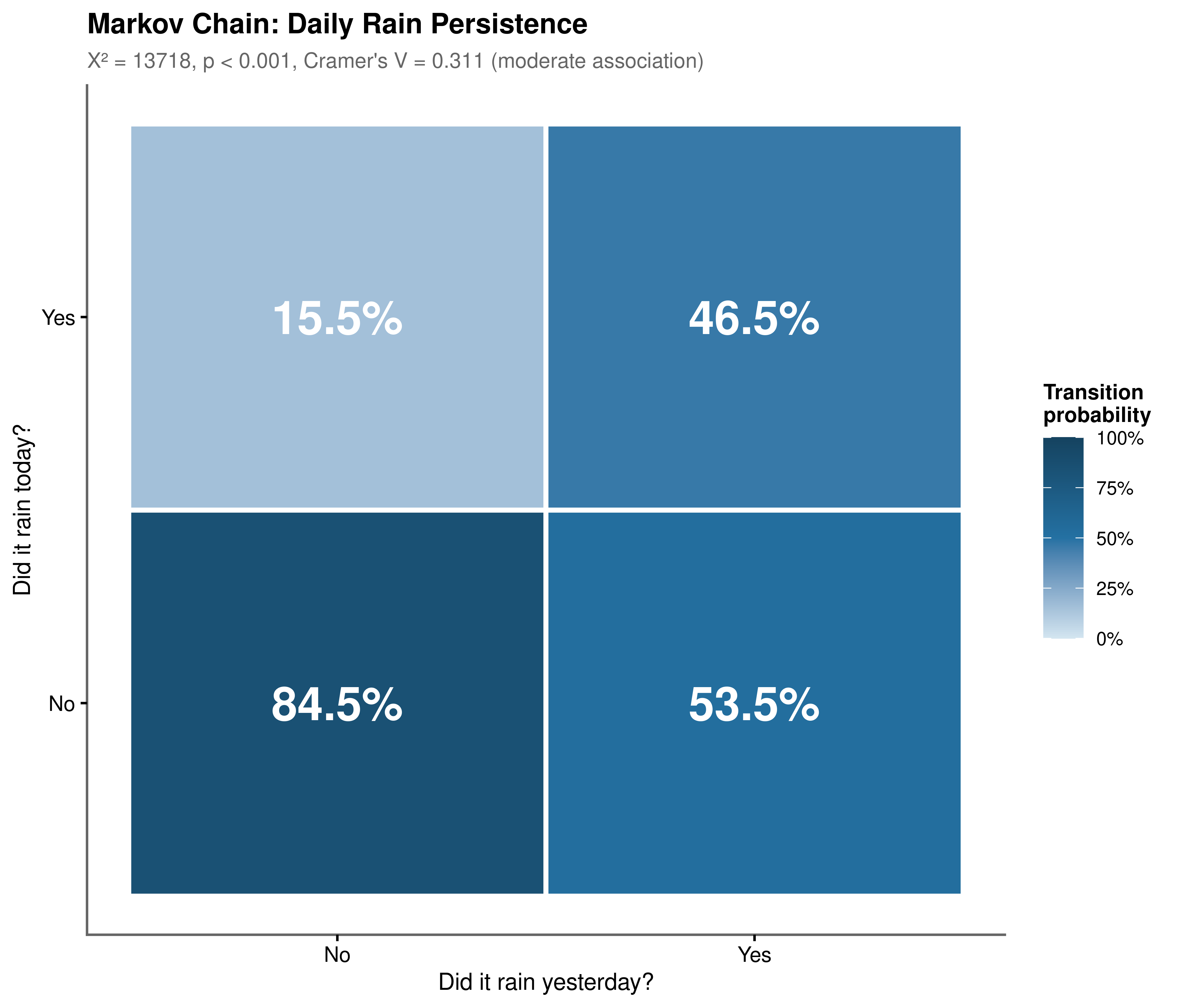

Show the code

markov_stats <- run_markov_stats(cont_table)
#> 
#> Effect Size Interpretation
#> V = 0.3107: Moderate Association

Show the code

plot_markov_chain(markov_stats = markov_stats)

Figure 4.2: Markov chain transition matrix. The asymmetry between dry-to-dry (85%) and wet-to-wet (47%) probabilities is the central finding: dry states are self-reinforcing while wet states are more transient.

The Chi-squared test yields \(\chi^2 \approx 13{,}718\), \(p < 0.001\), rejecting daily independence by a wide margin. Cramer’s \(V \approx 0.31\) confirms a moderate practical effect size.

The transition matrix (Figure 4.2) reveals an important asymmetry. When the previous day was dry, there is an 85% probability of remaining dry: high-pressure systems are persistent and self-reinforcing. When the previous day was wet, there is only a 47% probability of continued rain, meaning wet events are considerably more transient. This asymmetry has a direct atmospheric interpretation: anticyclonic systems can persist for days to weeks, while frontal systems typically pass through more quickly.

rain_today (lagged one day) carries meaningful predictive signal, yet its modest effect size also demonstrates that autocorrelation alone is insufficient. The wet state is too transient for a persistence-only rule, and other meteorological covariates remain necessary.

4.4.3 Dry Spell Dynamics and Temporal Decay

Show the code

dry_spell_dat <- build_dry_spell_data()

Show the code

dry_spell_models <- run_dry_spell_models(dry_spell_dat)
#> Wald test:
#> ----------
#> 
#> Chi-squared test:
#> X2 = 8099.7, df = 1, P(> X2) = 0.0
#> 
#> For each additional day without rain, odds of rainfall decrease by 16.5%
#> 95% CI: [0.831, 0.838]
#> Analysis of Deviance Table
#> 
#> Model 1: rain_binary ~ days_since_rain
#> Model 2: rain_binary ~ splines::ns(days_since_rain, df = 4)
#>   Resid. Df Resid. Dev Df Deviance  Pr(>Chi)    
#> 1    138444     169706                          
#> 2    138441     162027  3   7678.7 < 2.2e-16 ***
#> ---
#> Signif. codes:  0 '***' 0.001 '**' 0.01 '*' 0.05 '.' 0.1 ' ' 1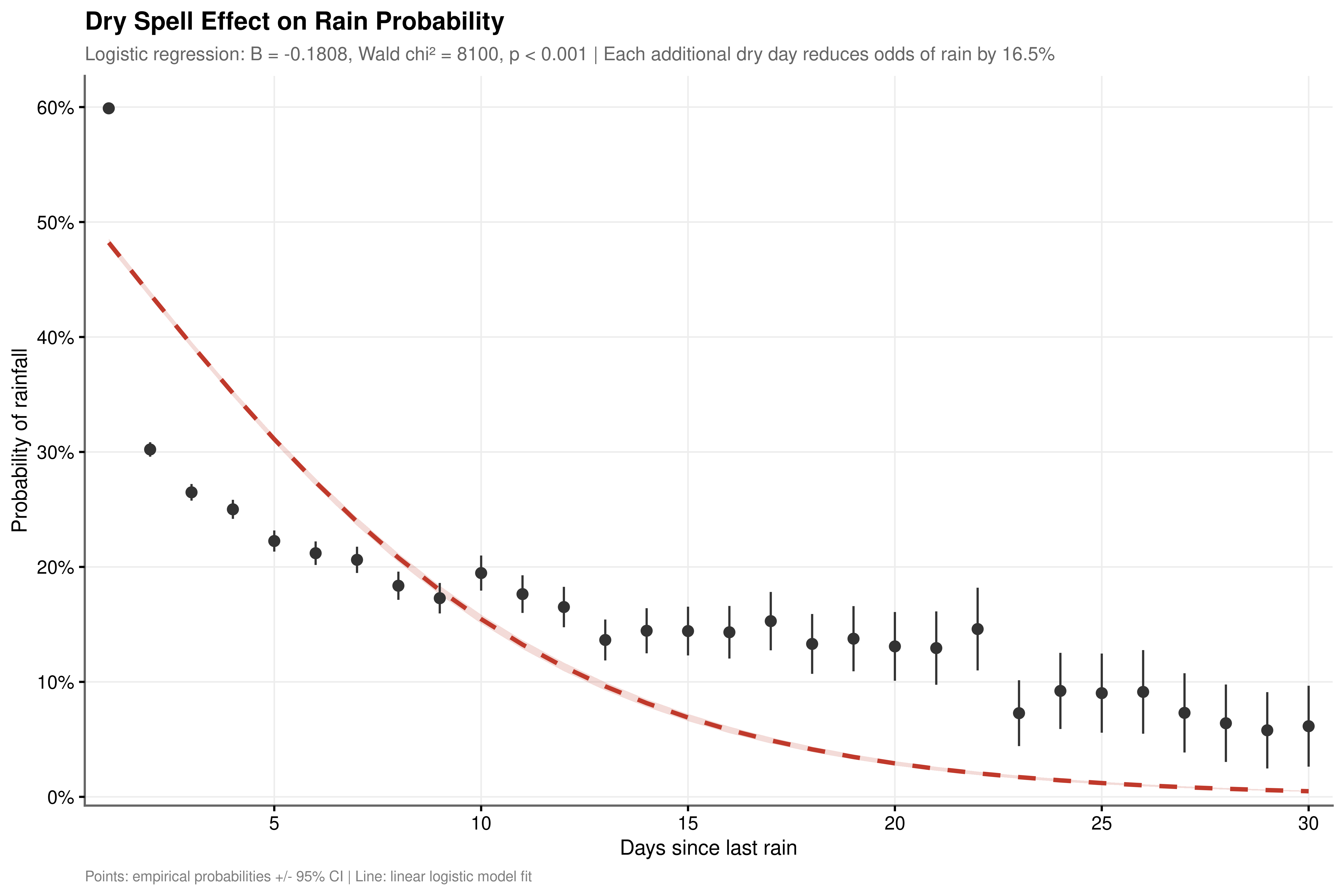

Show the code

plot_dry_spell(dry_spell_dat, dry_spell_models)

Figure 4.3: Probability of rainfall by days since last rain. Points are empirical probabilities (plus or minus 95% CI); the dashed line and shaded band show the linear logistic model fit and its uncertainty. The steep initial decline followed by a plateau motivates a spline parameterisation rather than a linear logistic term.

A logistic regression of daily rain occurrence on days_since_rain yields \(OR = 0.835\) (Wald \(\chi^2 \approx 8{,}099\), \(p < 0.001\)): each additional dry day reduces the odds of rainfall by approximately 16.5%. This is consistent with the progressive establishment of stable high-pressure ridges documented in the Markov analysis above.

The linear model is an approximation. A likelihood ratio test against a four-knot natural spline is highly significant (\(\chi^2 \approx 7{,}678\), \(p < 0.001\)). The empirical pattern (Figure 4.3) shows rain probability falling sharply from approximately 48% on Day 1 to around 18% by Day 10, then plateauing in the 12 to 16% range through Days 15 to 30. The linear model underestimates the initial steepness and overestimates the long-drought decline rate. This rapid-then-gradual decay motivates a spline parameterisation of days_since_rain rather than a simple linear term.

4.5 Atmospheric Pressure Dynamics

Show the code

source(here::here("chapter4", "pressure.R"))
pressure_dat <- build_pressure_data()
plot_pressure_qq(pressure_dat)

Show the code

render_pressure_ttests(pressure_dat)

Table 4.7: Welch two-sample t-test results for pressure metrics by rainfall state (Bonferroni-Holm corrected).

Welch Two-Sample t-test Results (Bonferroni-Holm Corrected)
Metric	Group 1	Group 2	t-statistic	df	Significance
pressure3pm	No	Yes	34.656	47862.40	****
pressure9am	No	Yes	63.848	47259.23	****
pressure_change	No	Yes	-73.395	46002.79	****

Show the code

render_pressure_cohens_d(pressure_dat)

Table 4.8: Cohen’s d effect size analysis for pressure metrics by rainfall state.

Cohen's d Effect Size Analysis
Metric	Effect Size (d)	Interpretation
pressure3pm	0.227	Small
pressure9am	0.419	Small
pressure_change	-0.487	Small

Show the code

plot_pressure_violin(pressure_dat)

Figure 4.4: Violin plots of atmospheric pressure variables by rainfall state. The pressure_change panel shows the most pronounced separation between dry and rainy days.

Show the code

plot_pressure_means()

Figure 4.5: Mean pressure levels and diurnal drop by rainfall state. The suppressed diurnal pressure drop on rainy days relative to dry days is a stronger discriminating signal than the absolute pressure baseline.

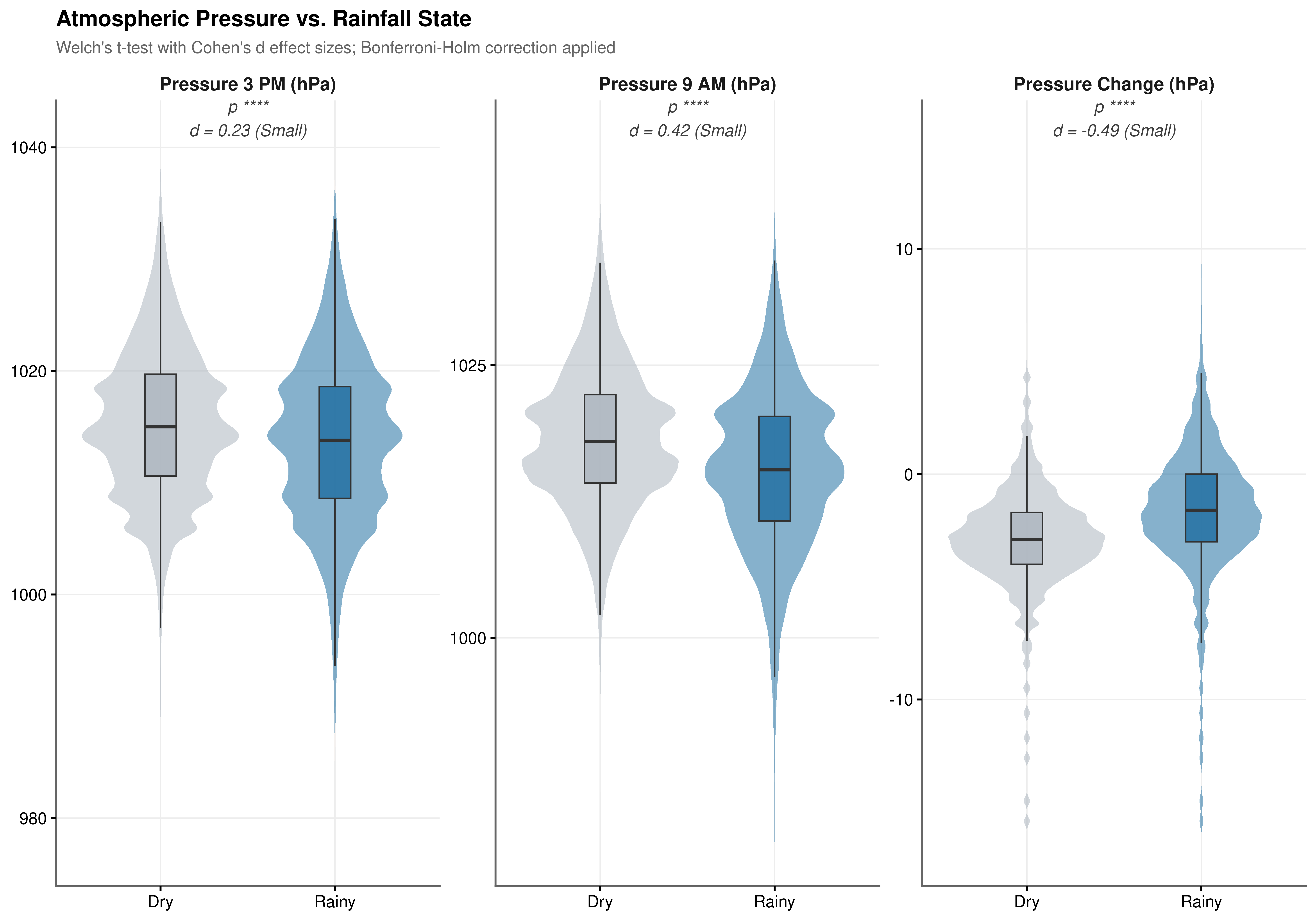
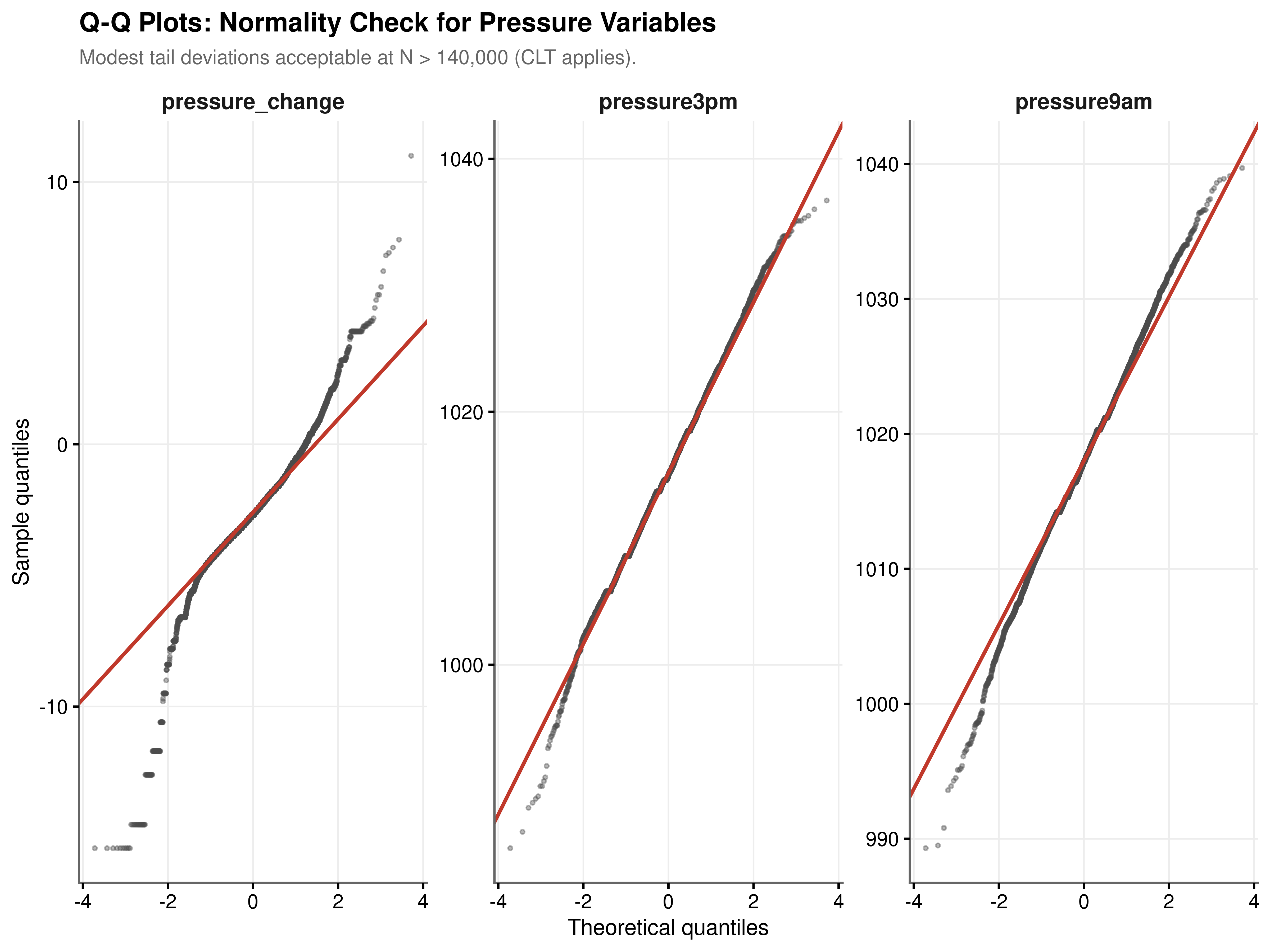
Normality and Test Validity. Q-Q plots reveal modest tail deviations across all three pressure metrics, but with \(N > 140{,}000\) the Central Limit Theorem ensures that sample means are asymptotically normal regardless of the underlying marginal distribution. Welch’s t-test is used throughout to avoid the equal-variance assumption, and Bonferroni-Holm correction is applied across the three comparisons.

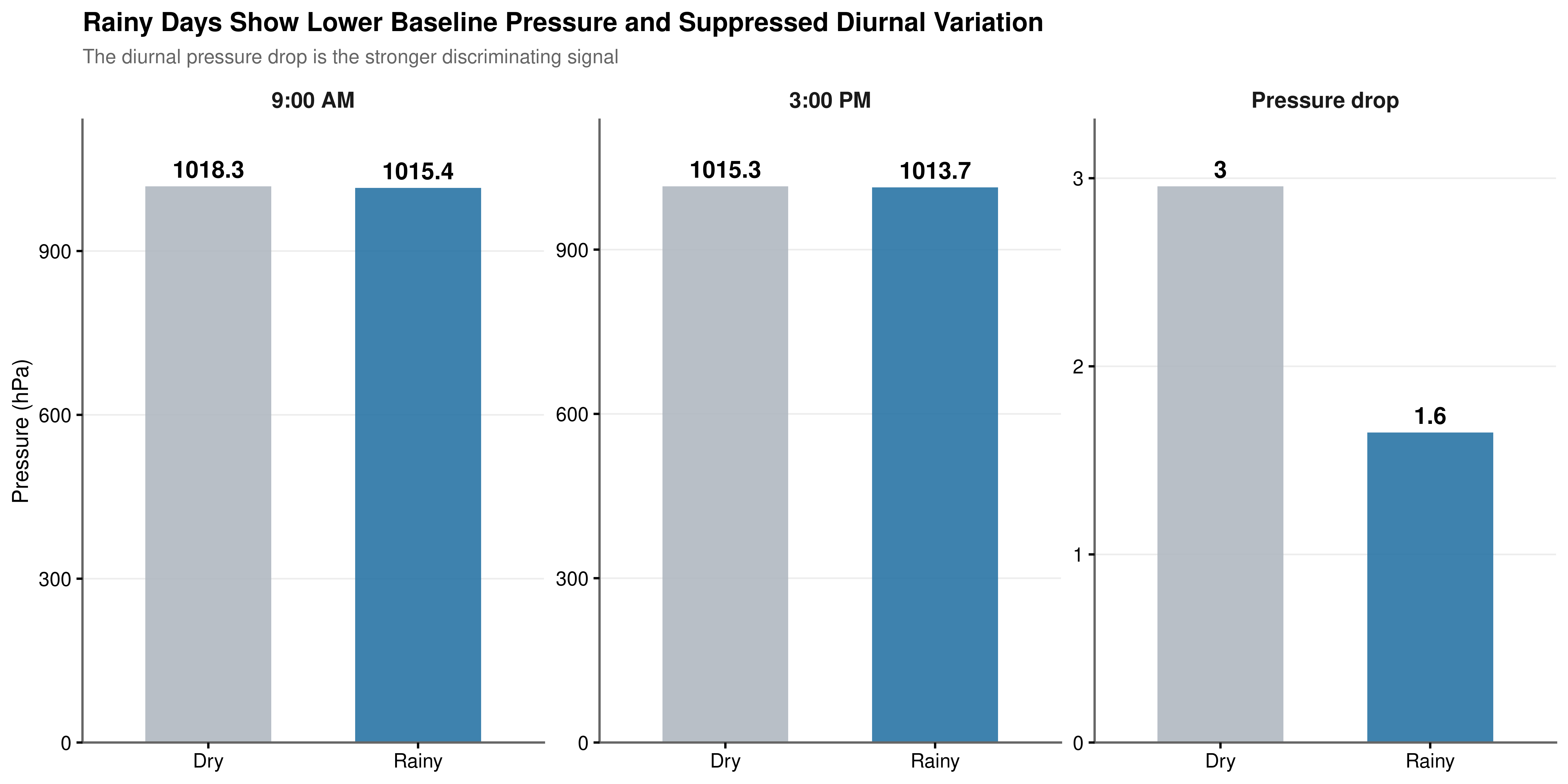
Baseline Pressure. Rainy days show significantly lower mean atmospheric pressure than dry days at both observation times (Table 4.7). Cohen’s \(d\) for the baseline measures ranges from 0.227 to 0.419, a small effect (Table 4.8). Lower absolute pressure is a necessary but not sufficient condition for rainfall: the overlap between the two distributions is substantial enough that pressure level alone cannot discriminate reliably between states.

Diurnal Pressure Change. The stronger discriminating signal lies not in the baseline but in how pressure evolves across the day (Figure 4.4, Figure 4.5). Cohen’s \(d = -0.487\) for pressure_change exceeds the effect size of either absolute pressure reading, and the Welch t-statistic of \(-73.395\) is the largest in magnitude among all three metrics (Table 4.7, Table 4.8). The rate of pressure change across the day is therefore a more discriminating indicator of rainfall state than the morning or afternoon level in isolation, and it is entered as a primary derived feature in the engineering pipeline.

4.6 Seasonal Rainfall Intensity

4.6.1 Cyclical Patterns

Show the code

source(here::here("chapter4", "seasonality.R"))
seasonal_dat <- build_seasonal_data()
monthly_stats <- build_monthly_stats()

Show the code

plot_monthly_ridgeline()

Figure 4.6: Ridgeline plot of monthly log-rainfall distributions. Shifting peaks illustrate how rainfall intensity varies cyclically relative to the global median (dashed line). Solid vertical lines within each ridge mark the monthly median.

Show the code

plot_seasonal_facet(seasonal_dat)

Show the code

plot_mean_rain_bar()

Figure 4.8: Mean rainfall intensity on non-zero days by month. February records the highest mean intensity at 10.1 mm, nearly double July’s 4.9 mm, illustrating that frequency and intensity vary in opposite directions across the seasonal cycle.

The frequency analysis in Section 4.4.1 established when rain tends to occur. This section investigates how much falls when it does.

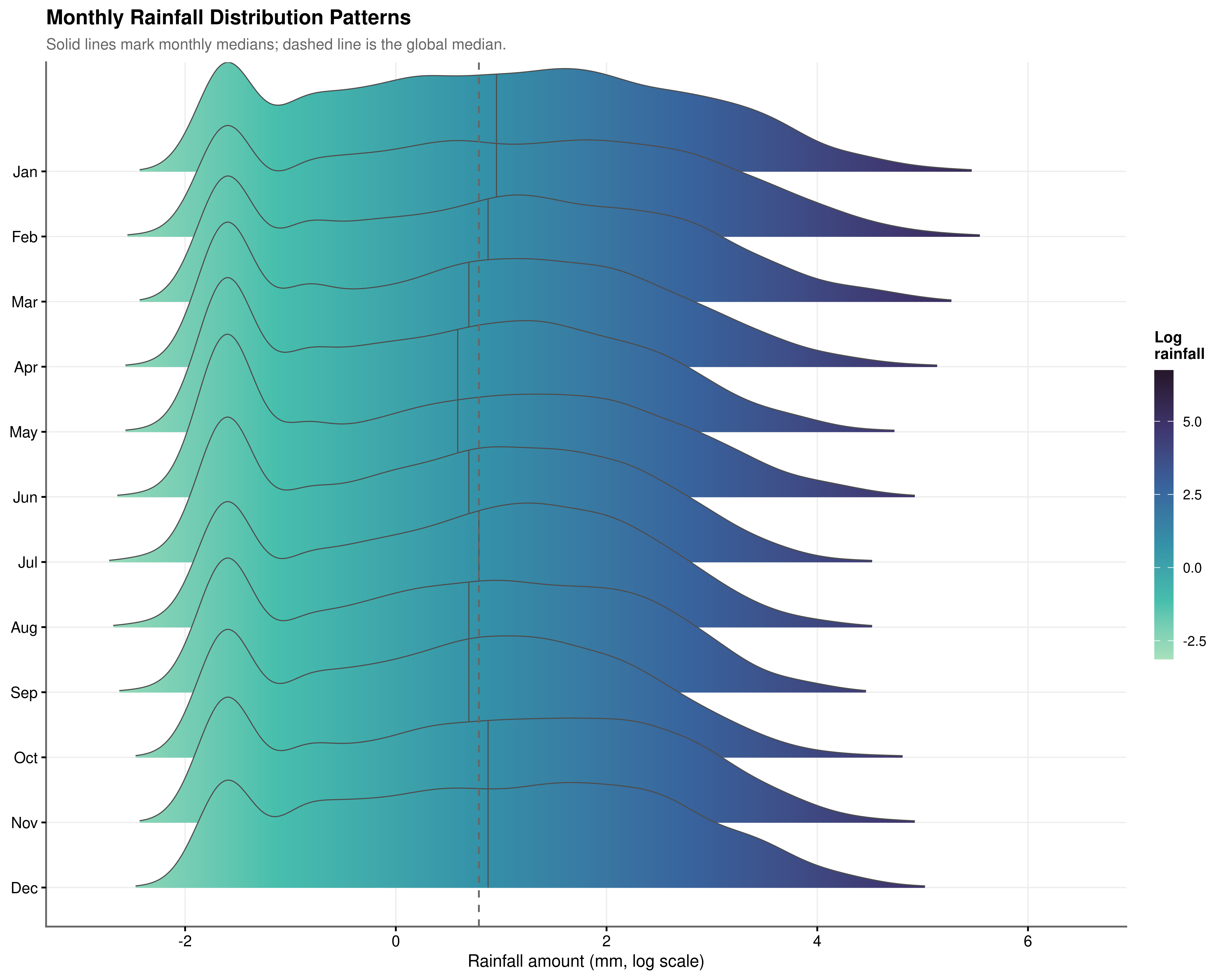
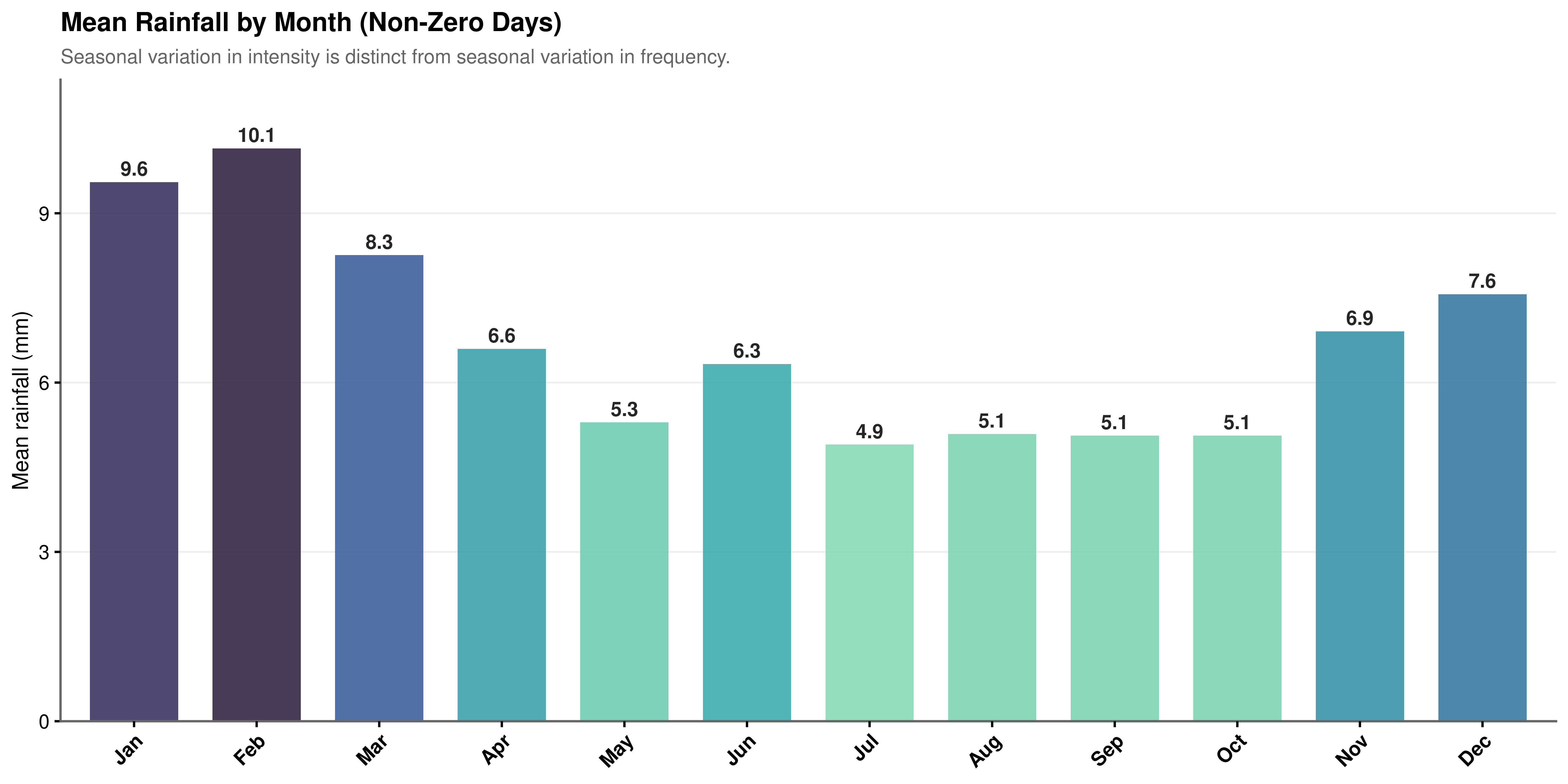
January and February distributions are shifted systematically right of the global median: summer storms are considerably more intense when they arrive, even though they occur less frequently. June through August cluster left, representing lower but more consistent rainfall. February records the highest mean intensity per wet day at 10.1 mm, nearly double July’s 4.9 mm (Figure 4.8).

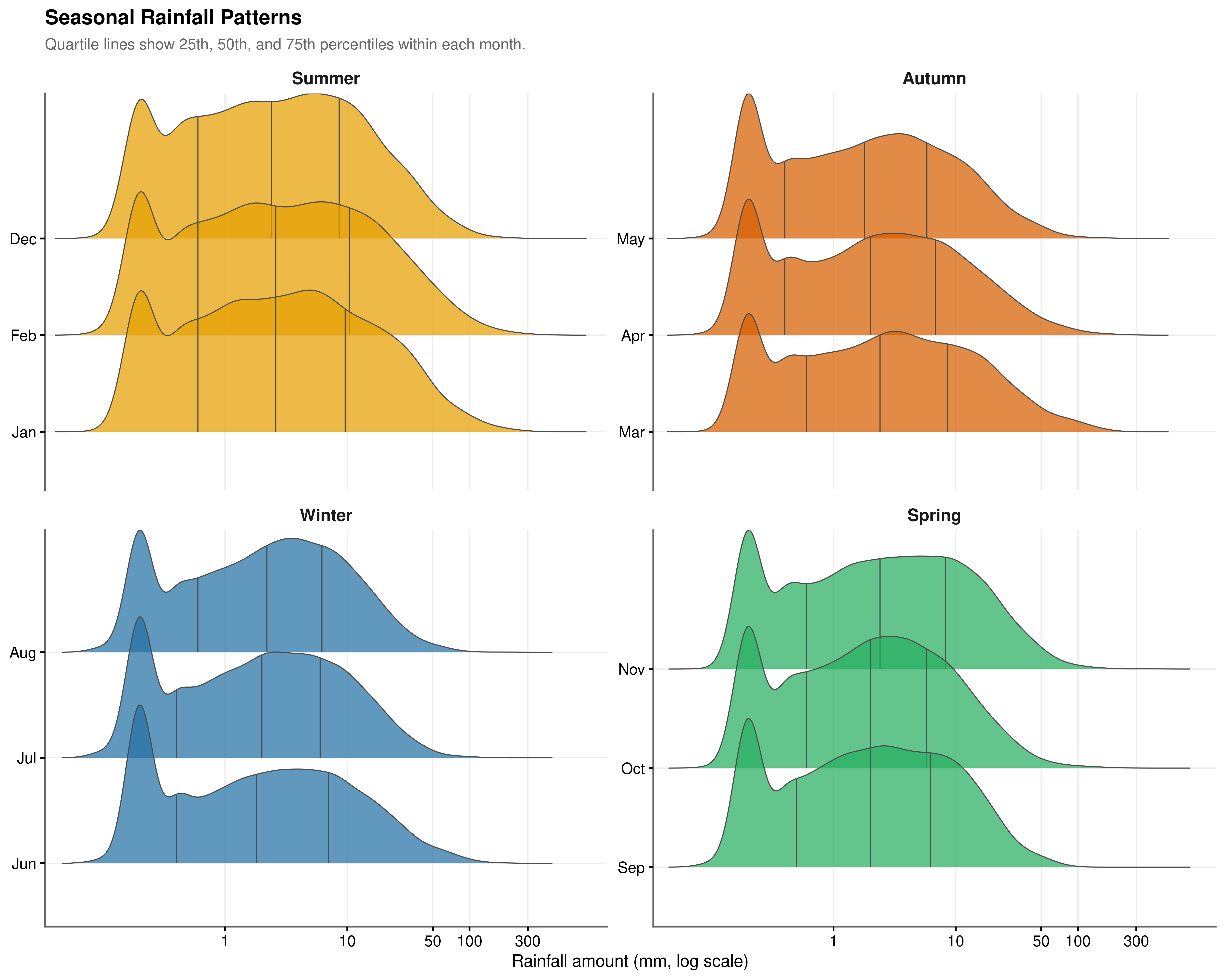
Summer rainfall has a wide interquartile range and a pronounced right tail beyond 100 mm per day, reflecting episodic convective storms (Figure 4.7). Winter shows a narrower, more peaked distribution. Both the frequency variation (more rain in winter) and the intensity variation (heavier rain in summer) carry independent information, and a complete model must account for both dimensions.

Encoding implication. Because the seasonal cycle is continuous, the transition from December to January is climatologically smooth, and treating Month as an unordered factor discards that proximity information. Cyclical encoding via sine and cosine transformations of the month number preserves the circular geometry of the annual cycle.

4.6.2 Statistical Validation

Show the code

render_seasonal_desc_stats(seasonal_dat)

Table 4.9: Descriptive statistics of rainfall intensity by meteorological season.

Descriptive Statistics of Rainfall Intensity by Season
Season	Variable	N (Events)	Mean (mm)	SD (mm)
Summer	rainfall	10571	9.070	18.195
Autumn	rainfall	13382	6.667	13.495
Winter	rainfall	15402	5.463	9.809
Spring	rainfall	11764	5.651	10.495

Show the code

seasonal_tests <- run_seasonal_tests(seasonal_dat)
render_kruskal_table(seasonal_tests)

Table 4.10: Kruskal-Wallis test of seasonal differences in rainfall intensity.

Statistical Significance of Seasonal Differences (Non-Parametric)
Test	Chi-squared	df	P-value	Effect Size	Magnitude
Kruskal-Wallis Rank Sum Test	230.44	3	<0.001	0.0044	small
^* Effect size: Epsilon-squared.
^† Alpha = 0.05

Show the code

render_dunns_table(seasonal_tests)

Table 4.11: Dunn’s pairwise comparison test with Bonferroni correction.

Dunn's Pairwise Comparison Test (Bonferroni Corrected)
Group 1	Group 2	Z-Statistic	Adj. P-Value	Significance
Summer	Autumn	-11.468	0.000	****
Summer	Winter	-14.483	0.000	****
Summer	Spring	-11.049	0.000	****
Autumn	Winter	-2.851	0.026	*
Autumn	Spring	0.091	1.000	ns
Winter	Spring	2.846	0.027	*

Show the code

plot_seasonal_stat_groups(seasonal_dat, seasonal_tests)

Figure 4.9: Mean seasonal rainfall with statistical groupings. Shared letters above bars indicate seasons not significantly different from one another at the Bonferroni-corrected threshold (Dunn’s test, p < 0.05).

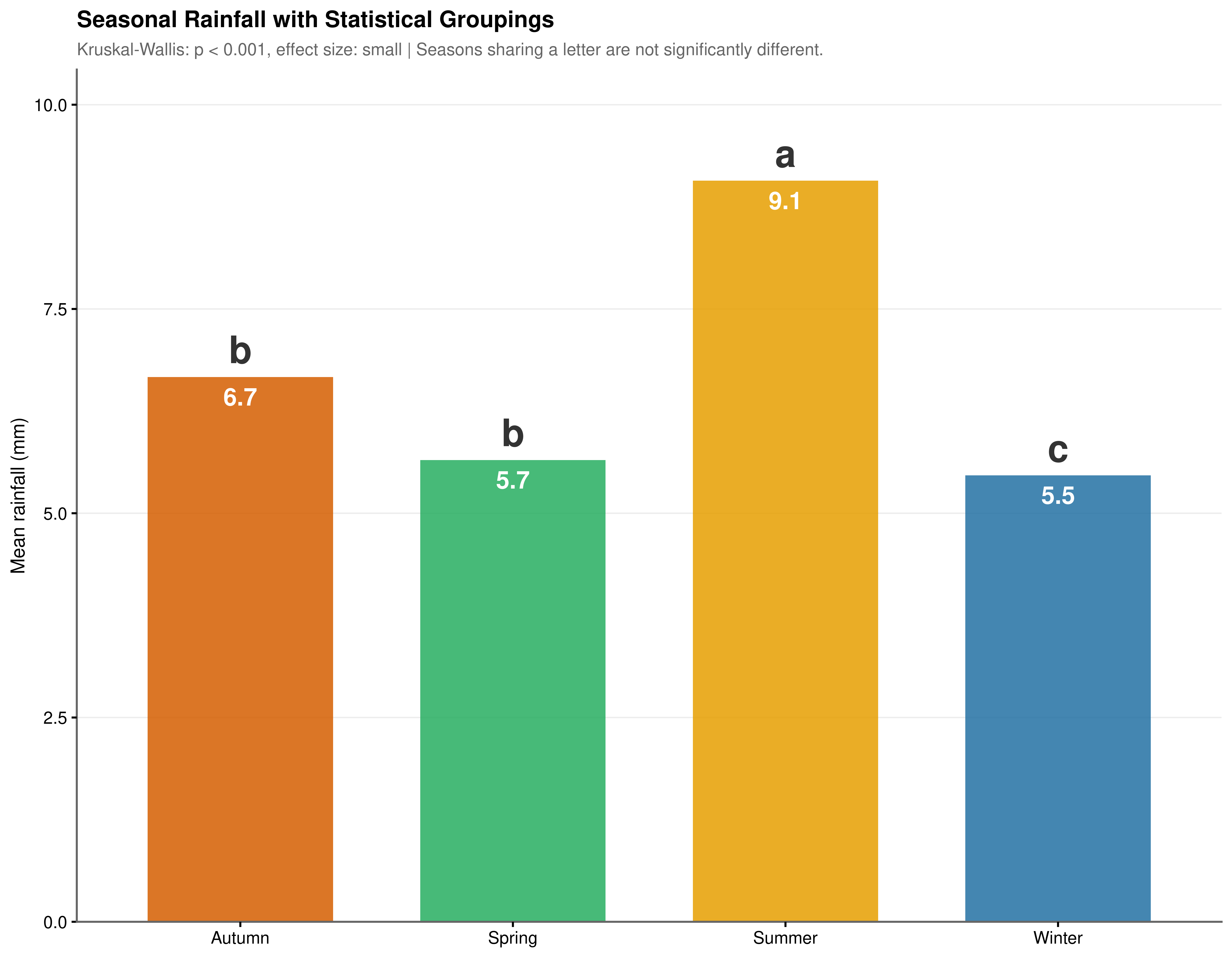
The Kruskal-Wallis test yields \(\chi^2 = 230.44\), \(p < 0.001\), strongly rejecting the null of equal seasonal distributions (Table 4.10). The epsilon-squared effect size (\(\eta^2 \approx 0.0044\)) is small: the seasonal signal is real but accounts for only a minor fraction of total variance in rainfall intensity, reinforcing the necessity of a multivariate approach.

Post-hoc Dunn’s tests identify three distinct statistical groups (Figure 4.9, Table 4.11). Summer stands alone as the most intense season (\(\bar{x} = 9.070\) mm, \(p < 0.001\) vs. all others). Autumn and Spring are statistically indistinguishable (\(p_\text{adj} = 1.000\)). Winter registers the lowest mean intensity (\(\bar{x} = 5.463\) mm) and is statistically distinct from Spring (\(p_\text{adj} = 0.027\)).

4.7 Feature Interactions: The “Rain Corner”

Show the code

source(here::here("chapter4", "interactions.R"))
plot_rain_corner()

Figure 4.10: Bivariate density of Humidity3pm versus Sunshine, faceted by rainfall occurrence. Rain events concentrate tightly in the upper-left corner (high humidity, low sunshine), while dry days are dispersed broadly across the feature space. This structural asymmetry justifies a multiplicative interaction term in the model specification.

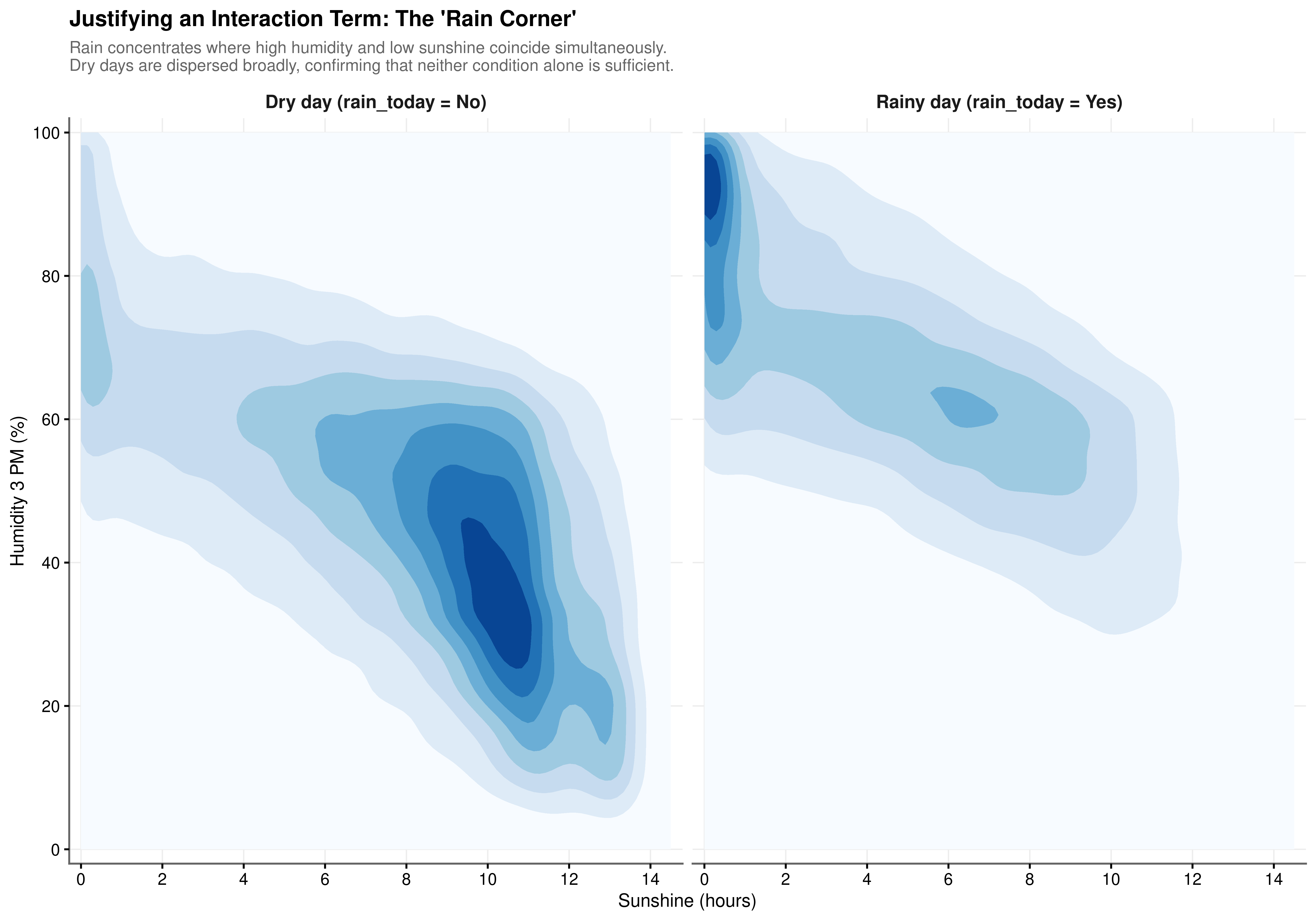
While individual correlation analysis in Section 4.3 identifies humidity and sunshine as primary predictors, a standard additive model assumes their effects on the log-odds of rainfall are independent. The bivariate density plots (Figure 4.10) test this assumption directly by visualising the joint distribution of these two features conditioned on the rainfall outcome.

Dry Day Structure. The feature space for dry days shows a concentrated region in the lower-right of the humidity-sunshine plane, where sunshine is moderate-to-high and afternoon humidity is low. This reflects the high-pressure suppression regimes documented in Section 4.4.2, where clear skies drive both elevated sunshine duration and suppressed humidity. Neither variable in isolation is a reliable discriminator between outcomes; the specific combination carries the predictive signal.

The Rain Corner. Precipitation events concentrate tightly in the upper-left quadrant of the feature space, where afternoon humidity is high and sunshine hours are low simultaneously. This cluster is not a feature of either variable’s marginal distribution: high humidity alone and low sunshine alone each occur on dry days with regularity. It is the joint occurrence that distinguishes the rainfall regime. The density mass that is dispersed broadly across the dry-day panel collapses into this single region when rain is present, a pattern that an additive model would be structurally unable to capture.

Modelling Implication. The asymmetry between the two panels confirms a genuine statistical interaction: the effect of humidity on rainfall probability is conditional on the level of sunshine, and vice versa. This justifies including a multiplicative interaction term (\(\text{Humidity3pm} \times \text{Sunshine}\)) in the model specification, in addition to both main effects.

4.8 Summary and Modelling Implications

The preceding analyses characterise the dataset along six interconnected dimensions, each producing a specific modelling requirement.

The distributional structure of the target variable; 64.05% zeros, extreme positive skew, and kurtosis of 181.146 rules out any single-component Gaussian model. A two-part framework separating occurrence from intensity is the appropriate response.

The missingness analysis (documented in Chapter 2, summarised in Section 4.1) establishes that imputation is necessary to preserve both sample size and the predictive signal in sunshine and evaporation, and that the predictive mean matching procedure does not introduce outcome-related bias. Downstream models incorporating these predictors must be fitted across all imputed completions and pooled via Rubin’s combining rules.

The correlation structure identifies humidity, cloud cover, sunshine, and evaporation as the strongest individual predictors, and flags severe multicollinearity among morning-afternoon pairs. VIF-based feature selection is required.

The temporal analyses establish that both the day-to-day Markov state and the cumulative dry spell duration carry predictive signal. Month should be cyclically encoded. The dry spell decay is non-linear and warrants a natural spline parameterisation of days_since_rain.

The pressure analysis identifies the diurnal pressure change as the more discriminating pressure-derived feature, with Cohen’s \(d = -0.487\) separating rainy from dry days more effectively than absolute pressure level.

The interaction analysis provides empirical justification for a \(\text{Humidity} \times \text{Sunshine}\) interaction term, reflecting the physical reality that precipitation concentrates where high moisture and low solar radiation coincide in the Rain Corner of the feature space.