Chapter3: Potential Outcomes and Counterfactuals

The Fundamental Problem

A potential outcome is what an outcome variable woult take under a specific exposure(treatment). Before treatmet occurs, every unit has one potential outcome per exposure level, \(Y(x)\) for each x. Once an exposure happens, only one potential outcome is realised. The rest are counterfactual ie they exist in the causal model but not in the data.

This is the fundamental problem of causal inference. The individual causal effect \(Y(X_{1})\) - \(Y(X_{0})\) requirs both potential outcomes simultaneously. You observe exactly one. Every method in the potential outomes framework is an attempt to use observed data to substitute for missing counterfactuals under explicit assumptions that justify the substitution.

Ice-T, Spike and the counterfactual proxy

The book opens with Ice-T and Spike, two men who grew upin the same Los Angeles gang neighborhoods, ran jewelry heists together, and then diverged. Ice-T was discovered rapping and left the criminal life; Spike continued and received a 35 years to life sentence. The premise is that each serves as the other’s counterfactual.

librarian::shelf(tidyverse, kableExtra)

tibble(person = c("Ice-T", "Spike"),
      path = c("Abandoned criminal life", "Continued criminal life"),
      outcome = c("Fame and Fortune", "35 years to life"),
      counterfactual_path = c("Did one more heist", "Abandoned Criminal Life"),
      missing_outcome = c("35 years to life", "Fame and fortune"))  |> 
      kbl(
      align = "lllll",
      col.names = c("Person", "Observed path", 
      "Observed outcome", "Counterfactual path", "Missing outcome")
      ) |>
      kable_styling(bootstrap_options = c("striped", "hover", "condensed"),
      full_width = FALSE,
      position = "left") |> 
      column_spec(1, bold = TRUE) |> 
      column_spec(4:5, color = "grey40", italic = TRUE) |> 
      add_header_above(c(" " = 3, "Counterfactual (unobservable)" = 2))

			Counterfactual (unobservable)
Person	Observed path	Observed outcome	Counterfactual path	Missing outcome
Ice-T	Abandoned criminal life	Fame and Fortune	Did one more heist	35 years to life
Spike	Continued criminal life	35 years to life	Abandoned Criminal Life	Fame and fortune

The premise is appealig but does not hold perfectly. Musical talent is a plausible cause of Ice-T’s outcome independent of his decision to quit, which makes Spike a reasonable proxy for what Ice-T would have faced had he continued, but not necessarily a symmetric counterfactual the other way round. This is the same asymmetry problem in every observational analysis. The chapter uses the story to motivate why we work with averaged effects over population rather than individual counterfactuals, and why randomization or adjustment is needed to construct valid proxies.

Potential Outcomes vs Counterfactuals

A Counterfactual is a potential outcome that was not realised, it’s counter to the fact of what happened. Potential outcomes are defined before the exposure, agnostic to what actually occurs. In practice, the book treats the two terms as interchangeable; once exposure has happened, you’re always looking at one realised outcome and at least one counter to the fact

The ice cream simulation

The oracle table: all potential outcomes known

Ten individuals each have a chocolate happiness score and a vanila happiness score. This “Oracle” view, both potential outcomes visible simultaneously, is never available in practice, it exists here only to define what we are trying to estimate.

library(tibble)
library(kableExtra)

# Save the tibble to a variable so we can reference it in row_spec
po_display <- po_data |>
  rename(
    ID                       = id,
    `Y(chocolate)`           = y_chocolate,
    `Y(vanilla)`             = y_vanilla,
    `Y(choc) - Y(van)`       = causal_effect
  )

po_display |>
  kbl(align = "cccc") |>
  kable_styling(
    bootstrap_options = c("striped", "hover", "condensed"),
    full_width        = FALSE,
    position          = "left"
  ) |>
  add_header_above(c(" " = 1, "Potential outcomes" = 2, "Individual causal effect" = 1)) |>
  row_spec(0, bold = TRUE) |>
  row_spec(which(po_display$`Y(choc) - Y(van)` < 0), color = "#c0392b") |>
  row_spec(nrow(po_display), bold = TRUE) |>
  footnote(
    general = paste0(
      "True ATE = ", round(mean(po_data$y_chocolate), 2),
      " - ", round(mean(po_data$y_vanilla), 2),
      " = ", round(mean(po_data$causal_effect), 2),
      ". Rows in red have negative individual causal effects (vanilla > chocolate for that person)."
    ),
    general_title = ""
  )

	Potential outcomes		Individual causal effect
ID	Y(chocolate)	Y(vanilla)	Y(choc) - Y(van)
1	4	1	3
2	4	3	1
3	6	4	2
4	5	5	0
5	6	5	1
6	5	6	-1
7	6	8	-2
8	7	6	1
9	5	3	2
10	6	5	1
True ATE = 5.4 - 4.6 = 0.8. Rows in red have negative individual causal effects (vanilla > chocolate for that person).

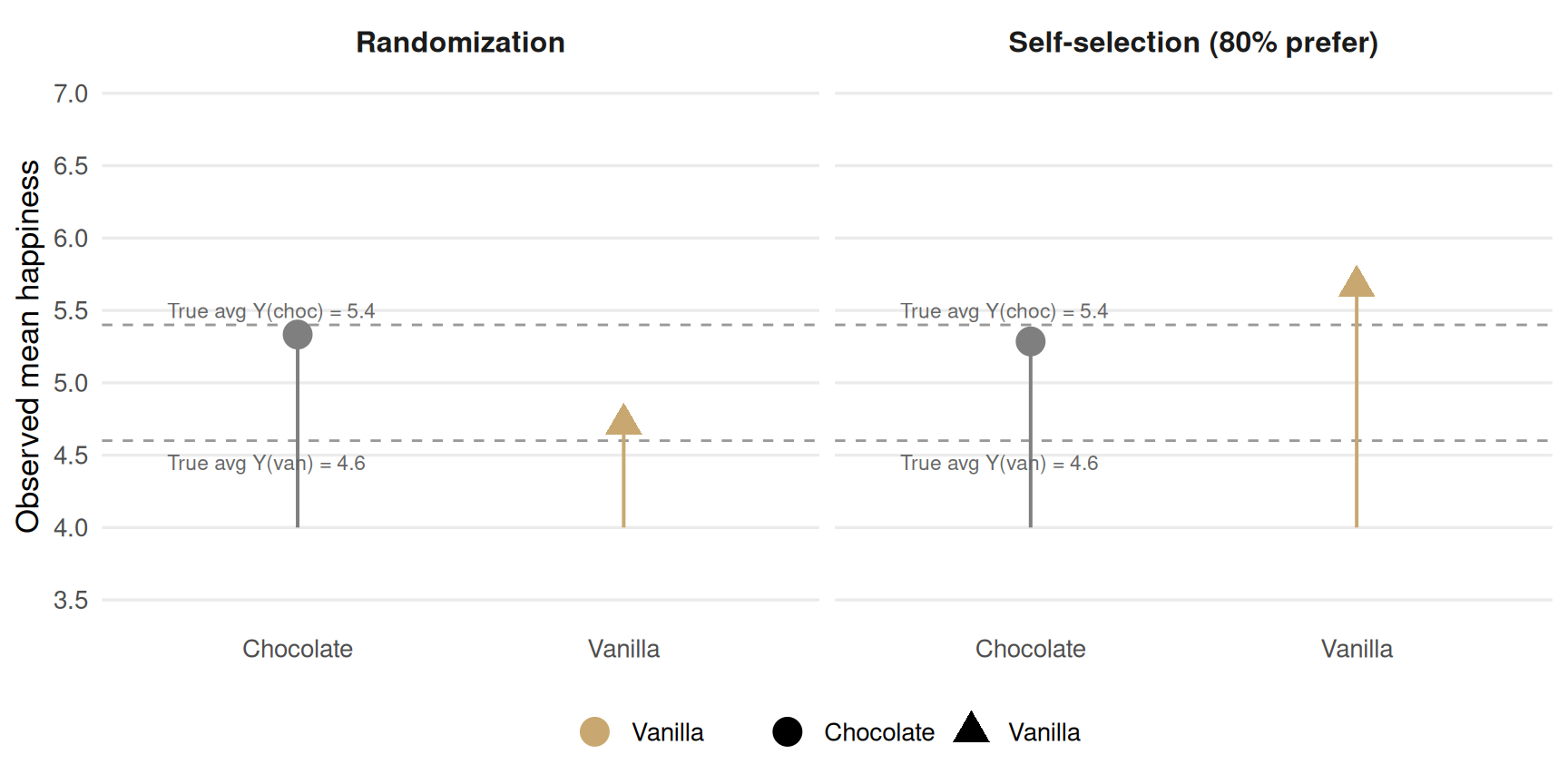
What we actually observe under randomization

Assign each participant randomly (50/50) to one flavor. Now only the assigned potential outcome is observed; the counterfactual is missing. Individual causal effects become unknowable.

set.seed(11)
observed_rand <- po_data |>
  mutate(
    exposure         = if_else(rbinom(n(), 1, 0.5) == 1, "chocolate", "vanilla"),
    observed_outcome = if_else(exposure == "chocolate", y_chocolate, y_vanilla),
    y_chocolate_disp = if_else(exposure == "chocolate", as.character(y_chocolate), "--"),
    y_vanilla_disp   = if_else(exposure == "vanilla",   as.character(y_vanilla),   "--")
  )

observed_rand |>
  select(
    ID                 = id,
    Exposure           = exposure,
    `Y(chocolate)`     = y_chocolate_disp,
    `Y(vanilla)`       = y_vanilla_disp,
    `Individual effect`= observed_outcome
  ) |>
  mutate(`Individual effect` = "--") |>
  kbl(align = "cclcc") |>
  kable_styling(
    bootstrap_options = c("striped", "hover", "condensed"),
    full_width        = FALSE,
    position          = "left"
  ) |>
  add_header_above(c(" " = 2, "Potential outcomes (one missing)" = 2, " " = 1)) |>
  row_spec(0, bold = TRUE) |>
  column_spec(2, bold = TRUE) |>
  column_spec(5, color = "grey50", italic = TRUE) |>
  footnote(
    general = paste0(
      "Observed ATE estimate = ",
      round(mean(observed_rand$observed_outcome[observed_rand$exposure == "chocolate"]), 2),
      " - ",
      round(mean(observed_rand$observed_outcome[observed_rand$exposure == "vanilla"]), 2),
      " = ",
      round(
        mean(observed_rand$observed_outcome[observed_rand$exposure == "chocolate"]) -
        mean(observed_rand$observed_outcome[observed_rand$exposure == "vanilla"]), 2
      ),
      ". Close to true ATE (0.8) due to randomization."
    ),
    general_title = ""
  )

		Potential outcomes (one missing)
ID	Exposure	Y(chocolate)	Y(vanilla)	Individual effect
1	vanilla	--	1	--
2	vanilla	--	3	--
3	chocolate	6	--	--
4	vanilla	--	5	--
5	vanilla	--	5	--
6	chocolate	5	--	--
7	vanilla	--	8	--
8	vanilla	--	6	--
9	chocolate	5	--	--
10	vanilla	--	5	--
Observed ATE estimate = 5.33 - 4.71 = 0.62. Close to true ATE (0.8) due to randomization.

Why Randomization Recovers ATE & self-selection destroys it

set.seed(113)
pref_obs <- po_data |>
  mutate(
    prefer_choc      = y_chocolate > y_vanilla,
    exposure         = case_when(
      prefer_choc  ~ if_else(rbinom(n(), 1, 0.8) == 1, "chocolate", "vanilla"),
      !prefer_choc ~ if_else(rbinom(n(), 1, 0.8) == 1, "vanilla",   "chocolate")
    ),
    observed_outcome = if_else(exposure == "chocolate", y_chocolate, y_vanilla)
  )

rand_means <- observed_rand |>
  summarise(mean_h = mean(observed_outcome), .by = exposure) |>
  mutate(mechanism = "Randomization")

pref_means <- pref_obs |>
  summarise(mean_h = mean(observed_outcome), .by = exposure) |>
  mutate(mechanism = "Self-selection (80% prefer)")

plot_means <- bind_rows(rand_means, pref_means) |>
  mutate(
    mechanism = factor(mechanism, levels = c("Randomization", "Self-selection (80% prefer)")),
    exposure  = str_to_title(exposure)
  )

ggplot(plot_means, aes(x = exposure, y = mean_h, colour = exposure, shape = exposure)) +
  geom_hline(yintercept = c(mean(po_data$y_chocolate), mean(po_data$y_vanilla)),
             linetype = "dashed", linewidth = 0.5, colour = "grey60") +
  geom_point(size = 5) +
  geom_segment(
    aes(xend = exposure, yend = 4),
    linewidth = 0.7, show.legend = FALSE
  ) +
  annotate("text", x = 0.6, y = mean(po_data$y_chocolate) + 0.1,
           label = "True avg Y(choc) = 5.4", hjust = 0, size = 3, colour = "grey40") +
  annotate("text", x = 0.6, y = mean(po_data$y_vanilla) - 0.15,
           label = "True avg Y(van) = 4.6", hjust = 0, size = 3, colour = "grey40") +
  facet_wrap(~mechanism) +
  scale_colour_manual(values = c(Chocolate = pal["chocolate"], Vanilla = "#c8a870"),
                      name = NULL) +
  scale_shape_manual(values = c(Chocolate = 19, Vanilla = 17), name = NULL) +
  scale_y_continuous(limits = c(3.5, 7), breaks = seq(3.5, 7, by = 0.5)) +
  labs(x = NULL, y = "Observed mean happiness") +
  theme_minimal(base_size = 13) +
  theme(
    panel.grid.major.x = element_blank(),
    panel.grid.minor   = element_blank(),
    strip.text         = element_text(face = "bold", size = 12),
    legend.position    = "bottom"
  )

Figure 4.1: Group mean happiness by flavor under randomization (left) and preference-driven self-selection (right). Under randomization the contrast recovers the true ATE; under self-selection it reverses sign.

ggplot(po_data, aes(x = causal_effect)) +
  geom_dotplot(
    binwidth   = 0.5,
    fill       = pal["observed"],
    colour     = "white",
    stackratio = 1.1
  ) +
  geom_vline(xintercept = mean(po_data$causal_effect),
             linetype = "dashed", linewidth = 0.8, colour = pal["unobserved"]) +
  annotate("text",
           x     = mean(po_data$causal_effect) + 0.12,
           y     = 0.9,
           label = paste0("ATE = ", round(mean(po_data$causal_effect), 1)),
           hjust = 0, size = 3.8, colour = pal["unobserved"]) +
  scale_x_continuous(breaks = -3:4, limits = c(-3, 4)) +
  scale_y_continuous(NULL, breaks = NULL) +
  labs(x = "Individual causal effect: Y(chocolate) - Y(vanilla)") +
  theme_minimal(base_size = 13) +
  theme(panel.grid.minor = element_blank())

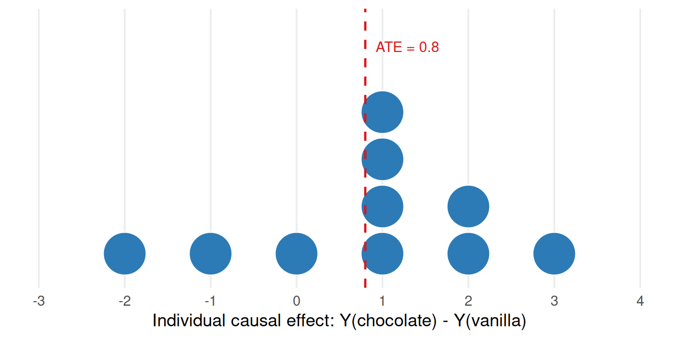
Figure 4.2: Distribution of individual causal effects from the oracle table. The ATE (0.8) is the mean, but individual effects range from -2 to +3. Negative effects (individuals who prefer vanilla) are the reason self-selection induces bias.

Causal Assumptions

For observed data to stand in missing counterfactuals, three identifiablity conditions have to hold. The book cals these the unconfoundedness assumptions, theyre required by the IPW, regression adjustment, g-computation, and most other methods covered. Miss one and you’re not estimating a causal effect anymore, whatever the statistics say.

tibble::tibble(
  Assumption     = c("Exchangeability", "Positivity", "Consistency"),
  `Also called`  = c(
    "No confounding; ignorability; unconfoundedness",
    "Probabilistic assumption; overlap",
    "SUTVA (Stable Unit Treatment Value Assumption)"
  ),
  `Formal notation` = c(
    "\\(Y(x) \\perp\\!\\!\\!\\perp X\\)",
    "\\(P(X = x) > 0\\) for all \\(x\\)",
    "\\(Y_{\\text{obs}} = X \\cdot Y(1) + (1-X) \\cdot Y(0)\\)"
  ),
  `Plain language` = c(
    "Exposure assignment is independent of potential outcomes",
    "Every unit has non-zero probability of each exposure level",
    "Observed outcome = potential outcome under received exposure"
  )
) |>
  kbl(
    escape   = FALSE,
    align    = c("l", "l", "c", "l"),
    booktabs = TRUE
  ) |>
  kable_styling(
    bootstrap_options = c("striped", "hover", "condensed"),
    full_width        = TRUE
  ) |>
  column_spec(1, bold = TRUE) |>
  column_spec(3, monospace = TRUE)

Table 4.1: The three core identifiability conditions for unconfoundedness methods.

Assumption	Also called	Formal notation	Plain language
Exchangeability	No confounding; ignorability; unconfoundedness	\(Y(x) \perp\!\!\!\perp X\)	Exposure assignment is independent of potential outcomes
Positivity	Probabilistic assumption; overlap	\(P(X = x) > 0\) for all \(x\)	Every unit has non-zero probability of each exposure level
Consistency	SUTVA (Stable Unit Treatment Value Assumption)	\(Y_{\text{obs}} = X \cdot Y(1) + (1-X) \cdot Y(0)\)	Observed outcome = potential outcome under received exposure

The apples-to-apples principle

All three assumptions exist to solve the same problem; making sure the comparison groups are exchangeable, close enough that each can reasonably stand in for the other’s counterfactual. English speakers say “comparing apples to oranges”; other languages have their own versions:

• Cheese and Chalk (UK)
• Grandmothers and toads (Serbian)
• Potatoes and sweet potatoes (Latin American Spanish)

The diagnostic question: do the groups differ in ways that are tied to both the exposure and the outcome? If yes, the comparison is broken before any statistics happen

Exchangeability

What exchangeability looks like and what breaks it

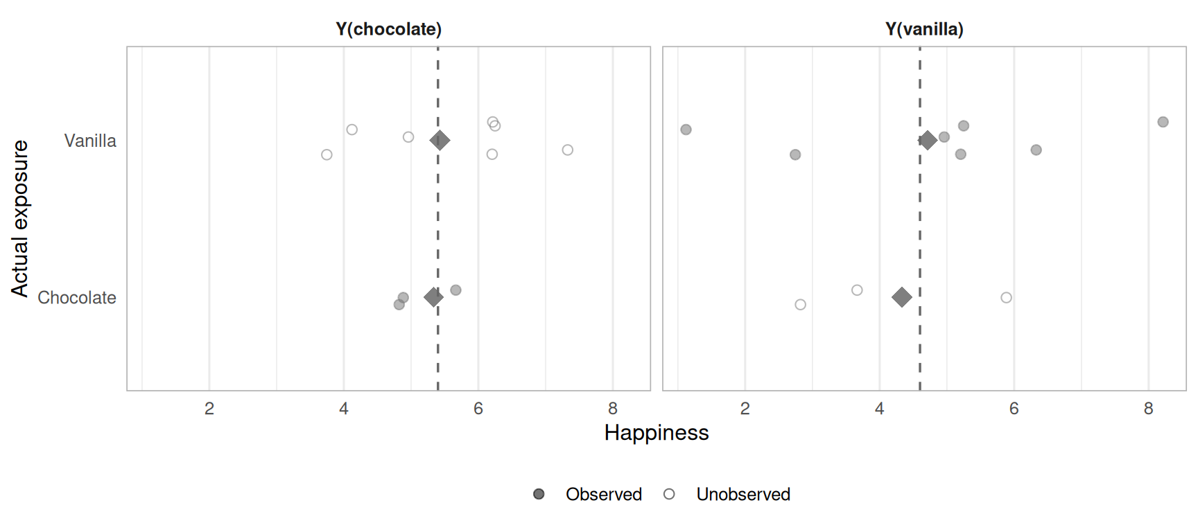
Under randomization, the two groups have the same distribution of potential outcomes on average. The observed average of \(Y_{i}(Chocolate)\) in the chocolate group is an unbiased estimate of the unobserved average of \(Y_{i}(Chocolate)\) in the vanilla group, and vice versa. This is the key to recovering ATE.

rand_long <- observed_rand |>
  pivot_longer(
    cols         = c(y_chocolate, y_vanilla),
    names_to     = "po",
    names_prefix = "y_",
    values_to    = "happiness"
  ) |>
  mutate(
    observed     = if_else(exposure == po, "Observed", "Unobserved"),
    po_lbl       = str_c("Y(", po, ")"),
    exposure_lbl = str_to_title(exposure)
  )

true_means <- tibble(
  po_lbl = c("Y(chocolate)", "Y(vanilla)"),
  truth  = c(mean(po_data$y_chocolate), mean(po_data$y_vanilla))
)

avg_rand <- rand_long |>
  summarise(mean_h = mean(happiness), .by = c(po_lbl, exposure_lbl, observed))

ggplot(rand_long, aes(x = happiness, y = exposure_lbl,
                      colour = observed, shape = observed)) +
  geom_jitter(height = 0.12, alpha = 0.55, size = 2.2) +
  geom_point(
    data    = avg_rand,
    mapping = aes(x = mean_h, y = exposure_lbl, colour = observed),
    shape   = 18, size = 5, inherit.aes = FALSE
  ) +
  geom_vline(
    data    = true_means,
    mapping = aes(xintercept = truth),
    linetype = "dashed", linewidth = 0.6, colour = "grey40"
  ) +
  facet_wrap(~po_lbl) +
  scale_colour_manual(
    values = c("Observed" = pal["observed"], "Unobserved" = pal["unobserved"]),
    name   = NULL
  ) +
  scale_shape_manual(values = c("Observed" = 19, "Unobserved" = 1), name = NULL) +
  labs(x = "Happiness", y = "Actual exposure") +
  theme_minimal(base_size = 12) +
  theme(
    panel.grid.major.y = element_blank(),
    panel.border       = element_rect(colour = "grey70", fill = NA, linewidth = 0.6),
    strip.text         = element_text(face = "bold"),
    legend.position    = "bottom"
  )

Figure 4.3: Potential outcomes by exposure group under randomization. Both groups’ observed averages (filled diamonds) are close to the true marginal means (dashed lines), confirming exchangeability.

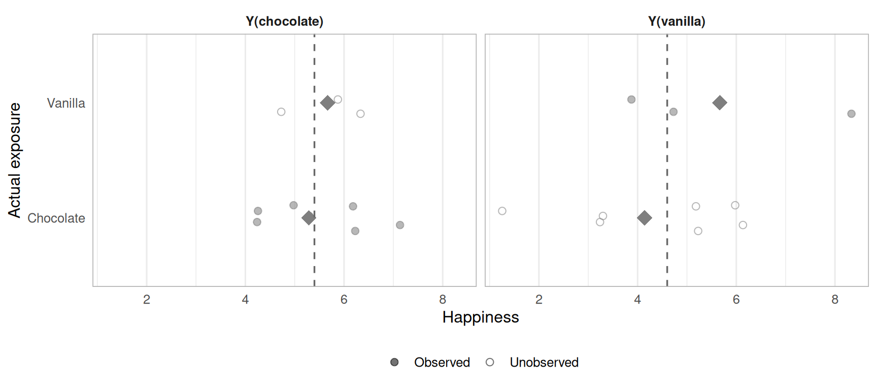
Under self-selection, people choose the flavor they prefer 80% of the time. Now Y(vanilla) averages diverge sharply by group, the chocolate group(who mostly prefer chocolate and avoided vanilla) has lower observed Y(vanilla) than the vanilla group. The groups are no longer exhangeable

set.seed(113)
pref_long <- pref_obs |>
  pivot_longer(
    cols         = c(y_chocolate, y_vanilla),
    names_to     = "po",
    names_prefix = "y_",
    values_to    = "happiness"
  ) |>
  mutate(
    observed     = if_else(exposure == po, "Observed", "Unobserved"),
    po_lbl       = str_c("Y(", po, ")"),
    exposure_lbl = str_to_title(exposure)
  )

avg_pref <- pref_long |>
  summarise(mean_h = mean(happiness), .by = c(po_lbl, exposure_lbl, observed))

ggplot(pref_long, aes(x = happiness, y = exposure_lbl,
                      colour = observed, shape = observed)) +
  geom_jitter(height = 0.12, alpha = 0.55, size = 2.2) +
  geom_point(
    data    = avg_pref,
    mapping = aes(x = mean_h, y = exposure_lbl, colour = observed),
    shape   = 18, size = 5, inherit.aes = FALSE
  ) +
  geom_vline(
    data    = true_means,
    mapping = aes(xintercept = truth),
    linetype = "dashed", linewidth = 0.6, colour = "grey40"
  ) +
  facet_wrap(~po_lbl) +
  scale_colour_manual(
    values = c("Observed" = pal["observed"], "Unobserved" = pal["unobserved"]),
    name   = NULL
  ) +
  scale_shape_manual(values = c("Observed" = 19, "Unobserved" = 1), name = NULL) +
  labs(x = "Happiness", y = "Actual exposure") +
  theme_minimal(base_size = 12) +
  theme(
    panel.grid.major.y = element_blank(),
    panel.border       = element_rect(colour = "grey70", fill = NA, linewidth = 0.6),
    strip.text         = element_text(face = "bold"),
    legend.position    = "bottom"
  )

Figure 4.4: Potential outcomes by exposure group under preference-driven self-selection. The Y(vanilla) averages differ markedly by group the chocolate group’s unobserved Y(vanilla) is systematically lower than the vanilla group’s. Exchangeability fails.

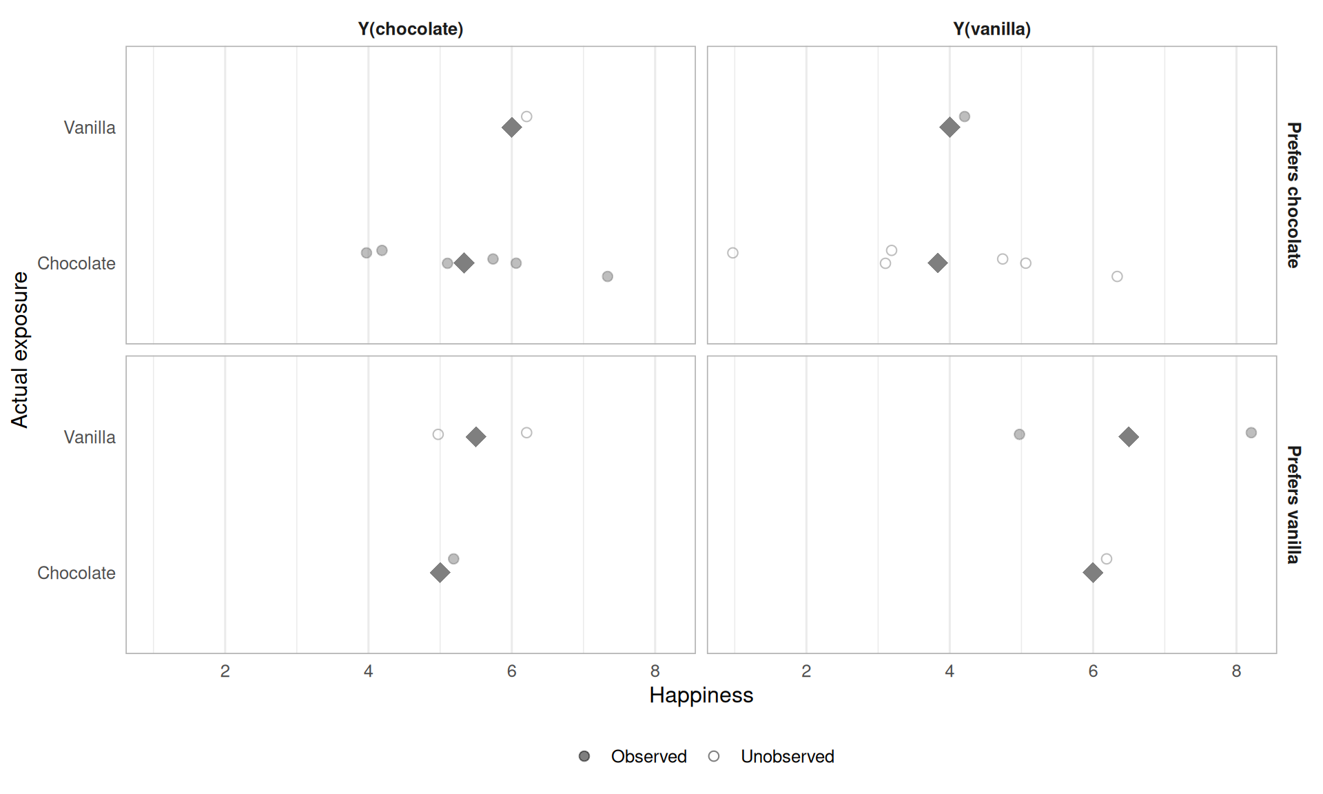
Conditional Exchangeability

Full exchangeability, \(Y(x) \\perp\\!\\!\\!\\perp X\), fails whenever exposure selection depends on potential outcomes. Conditional exchangeability, \(Y(x) \\perp\\!\\!\\!\\perp X | Z\), says the groups become exchangeable once you condition on Z. This is the operating assumption for all propensity score and regression adjustment methods.

pref_long2 <- pref_obs |>
  mutate(prefer_lbl = if_else(prefer_choc, "Prefers chocolate", "Prefers vanilla")) |>
  pivot_longer(
    cols         = c(y_chocolate, y_vanilla),
    names_to     = "po",
    names_prefix = "y_",
    values_to    = "happiness"
  ) |>
  mutate(
    observed     = if_else(exposure == po, "Observed", "Unobserved"),
    po_lbl       = str_c("Y(", po, ")"),
    exposure_lbl = str_to_title(exposure)
  )

avg_cond <- pref_long2 |>
  summarise(mean_h = mean(happiness), .by = c(po_lbl, exposure_lbl, prefer_lbl, observed))

ggplot(pref_long2, aes(x = happiness, y = exposure_lbl,
                       colour = observed, shape = observed)) +
  geom_jitter(height = 0.12, alpha = 0.5, size = 2.2) +
  geom_point(
    data    = avg_cond,
    mapping = aes(x = mean_h, y = exposure_lbl, colour = observed),
    shape   = 18, size = 5, inherit.aes = FALSE
  ) +
  facet_grid(prefer_lbl ~ po_lbl) +
  scale_colour_manual(
    values = c("Observed" = pal["observed"], "Unobserved" = pal["unobserved"]),
    name   = NULL
  ) +
  scale_shape_manual(values = c("Observed" = 19, "Unobserved" = 1), name = NULL) +
  labs(x = "Happiness", y = "Actual exposure") +
  theme_minimal(base_size = 12) +
  theme(
    panel.grid.major.y = element_blank(),
    panel.border       = element_rect(colour = "grey70", fill = NA, linewidth = 0.6),
    strip.text         = element_text(face = "bold"),
    legend.position    = "bottom"
  )

Figure 4.5: Potential outcomes by exposure group, stratified by flavor preference. Within each stratum, the two groups have similar potential outcome averages conditional exchangeability holds even when marginal exchangeability does not.

Its credibility depends entirely on whether Z captures all common causes of exposure and outcome. Unmeasured confounders break it, and unlike positivity (checkable empirically), conditional exchangeability is unverifiable from data alone.

Positivity

Stochastic positivity violation

With n = 10 and 80% self-selection, some covariate-exposure cells end up empty by chance. We need observations in every stratum to estimate stratum specific effects.

set.seed(1)
pos_data <- po_data |>
  mutate(
    prefer_choc = y_chocolate > y_vanilla,
    exposure    = case_when(
      prefer_choc  ~ if_else(rbinom(n(), 1, 0.8) == 1, "chocolate", "vanilla"),
      !prefer_choc ~ if_else(rbinom(n(), 1, 0.8) == 1, "vanilla",   "chocolate")
    )
  )

cell_counts <- pos_data |>
  count(prefer_choc, exposure) |>
  complete(
    prefer_choc,
    exposure = c("chocolate", "vanilla"),
    fill     = list(n = 0)
  ) |>
  mutate(
    prefer_lbl   = if_else(prefer_choc, "Prefers chocolate", "Prefers vanilla"),
    exposure_lbl = str_to_title(exposure),
    zero         = n == 0
  )

ggplot(cell_counts, aes(x = exposure_lbl, y = prefer_lbl, fill = n)) +
  geom_tile(colour = "white", linewidth = 1.2) +
  geom_text(aes(label = paste0("n = ", n),
                colour = if_else(zero, "white", "grey20")),
            size = 5, fontface = "bold") +
  scale_fill_gradient(
    low  = pal["unobserved"],
    high = "#d4e9f7",
    name = "Count"
  ) +
  scale_colour_identity() +
  labs(x = "Assigned exposure", y = NULL,
       title = "Stochastic positivity: cell counts under self-selection") +
  theme_minimal(base_size = 12) +
  theme(
    panel.grid   = element_blank(),
    axis.text    = element_text(size = 11),
    legend.position = "right"
  )

Figure 4.6: Cell counts for each preference-by-exposure combination under preference-driven self-selection. Empty cells (n = 0) are stochastic positivity violations, no observations exist to estimate potential outcomes in those strata.

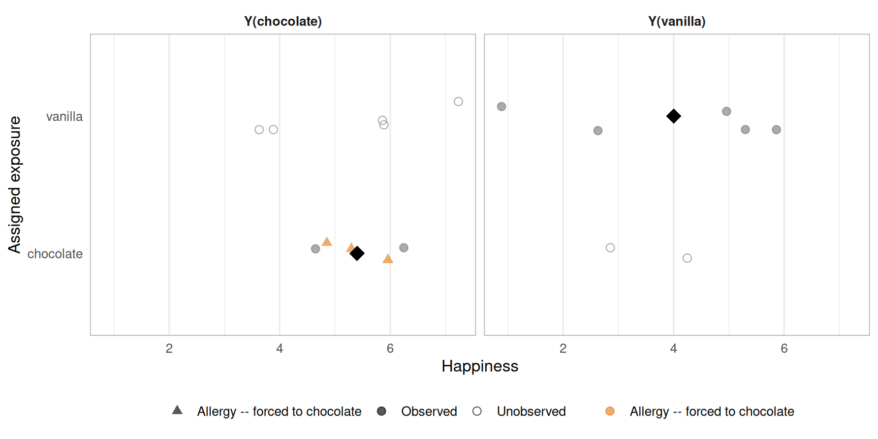
Structural positivity violation

Structural violations occur when some units literally cannot receive a given exposure level. Participants with a vanilla allergy cannot be assigned vanilla, Y(vanilla) is undefined for them, not merely unobserved.

set.seed(11)
struc_data <- po_data |>
  mutate(
    exposure = if_else(rbinom(n(), 1, 0.5) == 1, "chocolate", "vanilla")
  )

set.seed(1)
struc_data <- struc_data |>
  mutate(
    allergy          = rbinom(n(), 1, 0.3) == 1,
    exposure         = if_else(allergy, "chocolate", exposure),
    y_vanilla_adj    = if_else(allergy, NA_real_, y_vanilla),
    observed_outcome = if_else(exposure == "chocolate", y_chocolate, y_vanilla_adj)
  )

struc_long <- struc_data |>
  pivot_longer(
    cols      = c(y_chocolate, y_vanilla_adj),
    names_to  = "po",
    values_to = "happiness"
  ) |>
  mutate(
    po_lbl      = if_else(po == "y_chocolate", "Y(chocolate)", "Y(vanilla)"),
    observed    = case_when(
      po == "y_chocolate" & exposure == "chocolate" ~ "Observed",
      po == "y_vanilla_adj" & exposure == "vanilla" ~ "Observed",
      is.na(happiness) ~ "Undefined (allergy)",
      TRUE ~ "Unobserved"
    ),
    point_color = case_when(
      allergy & po == "y_chocolate" ~ "Allergy -- forced to chocolate",
      observed == "Observed"         ~ "Observed",
      observed == "Unobserved"       ~ "Unobserved",
      TRUE                           ~ "Undefined (allergy)"
    )
  )

avg_struc <- struc_long |>
  filter(observed == "Observed") |>
  summarise(mean_h = mean(happiness, na.rm = TRUE),
            .by = c(po_lbl, exposure))

ggplot(
  struc_long |> filter(!is.na(happiness)),
  aes(x = happiness, y = exposure, colour = point_color, shape = point_color)
) +
  geom_jitter(height = 0.12, alpha = 0.65, size = 2.5) +
  geom_point(
    data    = avg_struc,
    mapping = aes(x = mean_h, y = exposure),
    shape   = 18, size = 5, colour = "black", inherit.aes = FALSE
  ) +
  facet_wrap(~po_lbl) +
  scale_colour_manual(
    values = c(
      "Observed"                    = pal["observed"],
      "Unobserved"                  = pal["neutral"],
      "Allergy -- forced to chocolate" = "#e67e22"
    ),
    name = NULL
  ) +
  scale_shape_manual(
    values = c(
      "Observed"                    = 19,
      "Unobserved"                  = 1,
      "Allergy -- forced to chocolate" = 17
    ),
    name = NULL
  ) +
  labs(x = "Happiness", y = "Assigned exposure") +
  theme_minimal(base_size = 12) +
  theme(
    panel.grid.major.y = element_blank(),
    panel.border       = element_rect(colour = "grey70", fill = NA, linewidth = 0.6),
    strip.text         = element_text(face = "bold"),
    legend.position    = "bottom"
  )

Figure 4.7: Potential outcomes under a structural positivity violation. Individuals with a vanilla allergy (orange) have no Y(vanilla) counterpart the potential outcome is undefined, not missing at random. Their presence in the chocolate group inflates the estimated Y(chocolate) average.

tibble(
  Type    = c("Stochastic", "Structural"),
  Cause   = c(
    "Sampling variation produces empty exposure-covariate cells by chance",
    "Some units cannot receive at least one exposure level by biology or circumstance"
  ),
  Example = c(
    "With n = 10 and 80% self-selection, some preference-exposure strata end up with zero observations",
    "Participants with a vanilla allergy cannot receive vanilla; Y(vanilla) is undefined for them"
  ),
  Fix     = c(
    "Larger samples; propensity scores or g-computation to extrapolate over covariate dimensions",
    "Restrict eligibility criteria to exclude structurally ineligible units; modify the estimand to a population where positivity holds"
  )
) |>
  kbl(align = "llll") |>
  kable_styling(
    bootstrap_options = c("striped", "hover", "condensed"),
    full_width        = TRUE
  ) |>
  row_spec(0, bold = TRUE) |>
  column_spec(1, bold = TRUE, width = "9em") |>
  column_spec(2:4, width = "22em")

Table 4.2: Two forms of positivity violation

Type	Cause	Example	Fix
Stochastic	Sampling variation produces empty exposure-covariate cells by chance	With n = 10 and 80% self-selection, some preference-exposure strata end up with zero observations	Larger samples; propensity scores or g-computation to extrapolate over covariate dimensions
Structural	Some units cannot receive at least one exposure level by biology or circumstance	Participants with a vanilla allergy cannot receive vanilla; Y(vanilla) is undefined for them	Restrict eligibility criteria to exclude structurally ineligible units; modify the estimand to a population where positivity holds

Consistency

Consistency

Consistency requires that the observed outcome under X = x actually equals Y(x). It breaks in two ways.

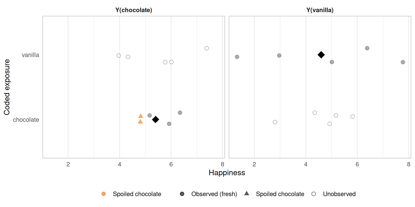
Poorly-defined exposure: spoiled chocolate

Two containers of chocolate exist, one fresh, one spoiled. Both are coded “chocolate.” The observed chocolate group is a mixture of Y(chocolate, spoiled = TRUE) and Y(chocolate, spoiled = FALSE), which have completely different potential outcomes.

pd_data <- po_data |>
  mutate(
    y_spoiled_choc = 0
  )

set.seed(11)
pd_obs <- pd_data |>
  mutate(
    true_exp = case_when(
      rbinom(n(), 1, 0.25) == 1 ~ "chocolate_spoiled",
      rbinom(n(), 1, 0.33) == 1 ~ "chocolate",
      TRUE                      ~ "vanilla"
    ),
    observed_outcome = case_when(
      true_exp == "chocolate_spoiled" ~ y_spoiled_choc,
      true_exp == "chocolate"         ~ y_chocolate,
      TRUE                            ~ y_vanilla
    ),
    exposure_coded = if_else(str_starts(true_exp, "chocolate"), "chocolate", "vanilla"),
    is_spoiled     = true_exp == "chocolate_spoiled"
  )

pd_long <- pd_obs |>
  pivot_longer(
    cols      = c(y_chocolate, y_vanilla),
    names_to  = "po",
    values_to = "happiness"
  ) |>
  mutate(
    po_lbl   = if_else(po == "y_chocolate", "Y(chocolate)", "Y(vanilla)"),
    observed = (exposure_coded == "chocolate" & po == "y_chocolate") |
               (exposure_coded == "vanilla"   & po == "y_vanilla"),
    pt_type  = case_when(
      is_spoiled & po == "y_chocolate" ~ "Spoiled chocolate",
      observed                          ~ "Observed (fresh)",
      TRUE                              ~ "Unobserved"
    )
  )

avg_pd <- pd_long |>
  filter(observed | (is_spoiled & po == "y_chocolate")) |>
  summarise(mean_h = mean(happiness), .by = c(po_lbl, exposure_coded))

ggplot(
  pd_long,
  aes(x = happiness, y = exposure_coded, colour = pt_type, shape = pt_type)
) +
  geom_jitter(height = 0.12, alpha = 0.65, size = 2.5) +
  geom_point(
    data    = avg_pd,
    mapping = aes(x = mean_h, y = exposure_coded),
    shape   = 18, size = 5, colour = "black", inherit.aes = FALSE
  ) +
  facet_wrap(~po_lbl) +
  scale_colour_manual(
    values = c(
      "Observed (fresh)"  = pal["observed"],
      "Spoiled chocolate" = "#e67e22",
      "Unobserved"        = pal["neutral"]
    ),
    name = NULL
  ) +
  scale_shape_manual(
    values = c(
      "Observed (fresh)"  = 19,
      "Spoiled chocolate" = 17,
      "Unobserved"        = 1
    ),
    name = NULL
  ) +
  labs(x = "Happiness", y = "Coded exposure") +
  theme_minimal(base_size = 12) +
  theme(
    panel.grid.major.y = element_blank(),
    panel.border       = element_rect(colour = "grey70", fill = NA, linewidth = 0.6),
    strip.text         = element_text(face = "bold"),
    legend.position    = "bottom"
  )

Figure 4.8: Potential outcomes under a poorly-defined exposure. The observed Y(chocolate) average (black diamond) is a blend of fresh-chocolate and spoiled-chocolate outcomes. Spoiled individuals (orange) drag the average down and make the estimate uninterpretable.

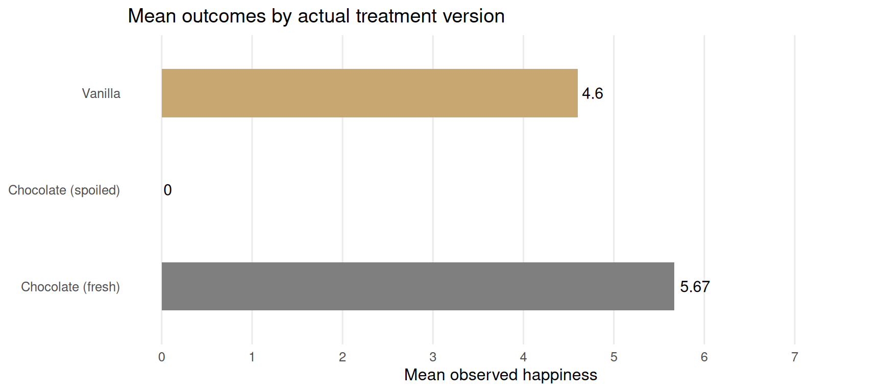
Stratifying by the actual exposure label (chocolate fresh / chocolate spoiled / vanilla) recovers the correct estimates.

pd_corrected <- pd_obs |>
  summarise(mean_outcome = mean(observed_outcome), .by = true_exp) |>
  mutate(
    true_exp = factor(true_exp,
                      levels = c("chocolate", "chocolate_spoiled", "vanilla"),
                      labels = c("Chocolate (fresh)", "Chocolate (spoiled)", "Vanilla"))
  )

ggplot(pd_corrected, aes(x = mean_outcome, y = true_exp, fill = true_exp)) +
  geom_col(width = 0.5, show.legend = FALSE) +
  geom_text(aes(label = round(mean_outcome, 2)), hjust = -0.2, size = 4) +
  scale_fill_manual(values = c(
    "Chocolate (fresh)"   = pal["chocolate"],
    "Chocolate (spoiled)" = "#e67e22",
    "Vanilla"             = "#c8a870"
  )) +
  scale_x_continuous(limits = c(0, 7.5), breaks = seq(0, 7, by = 1)) +
  labs(x = "Mean observed happiness", y = NULL,
       title = "Mean outcomes by actual treatment version") +
  theme_minimal(base_size = 12) +
  theme(panel.grid.major.y = element_blank(),
        panel.grid.minor   = element_blank())

Figure 4.9: Potential outcomes after correcting for treatment version. Separating fresh and spoiled chocolate recovers the true Y(chocolate) average. The three-group contrast is now interpretable.

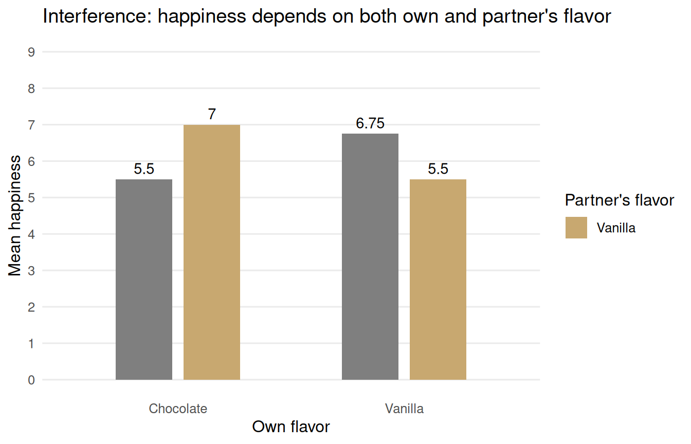
Interference: partner flavor effects

Each participant has a partner. Their happiness depends not only on their own flavor but also their partner’s, receiving a different flavor adds 2 happiness units. There are now four potential outcomes per person: Y(own, partner). A simple two-group contrast is estimating a mixture of these four quantities.

interf_data <- tibble(
  id                       = 1:10,
  partner_id               = c(1, 1, 2, 2, 3, 3, 4, 4, 5, 5),
  y_choc_choc              = c(4, 4, 6, 5, 6, 5, 6, 7, 5, 6),
  y_van_van                = c(1, 3, 4, 5, 5, 6, 8, 6, 3, 5)
) |>
  mutate(
    y_choc_van = y_choc_choc + 2,
    y_van_choc = y_van_van   + 2
  )

set.seed(37)
interf_obs <- interf_data |>
  mutate(
    own_exp     = if_else(rbinom(n(), 1, 0.5) == 1, "Chocolate", "Vanilla"),
    partner_exp = if_else(rbinom(n(), 1, 0.5) == 1, "Chocolate", "Vanilla"),
    observed    = case_when(
      own_exp == "Chocolate" & partner_exp == "Chocolate" ~ y_choc_choc,
      own_exp == "Chocolate" & partner_exp == "Vanilla"   ~ y_choc_van,
      own_exp == "Vanilla"   & partner_exp == "Chocolate" ~ y_van_choc,
      own_exp == "Vanilla"   & partner_exp == "Vanilla"   ~ y_van_van
    )
  )

interf_means <- interf_obs |>
  summarise(mean_h = mean(observed), .by = c(own_exp, partner_exp)) |>
  mutate(
    combo = str_c("Own: ", own_exp, "\nPartner: ", partner_exp)
  )

ggplot(interf_means, aes(x = own_exp, y = mean_h, fill = partner_exp)) +
  geom_col(position = position_dodge(width = 0.6), width = 0.5) +
  geom_text(
    aes(label = round(mean_h, 2)),
    position = position_dodge(width = 0.6),
    vjust    = -0.5,
    size     = 3.8
  ) +
  scale_fill_manual(
    values = c("Chocolate" = pal["chocolate"], "Vanilla" = "#c8a870"),
    name   = "Partner's flavor"
  ) +
  scale_y_continuous(limits = c(0, 9), breaks = seq(0, 9, by = 1)) +
  labs(
    x     = "Own flavor",
    y     = "Mean happiness",
    title = "Interference: happiness depends on both own and partner's flavor"
  ) +
  theme_minimal(base_size = 12) +
  theme(
    panel.grid.major.x = element_blank(),
    panel.grid.minor   = element_blank(),
    legend.position    = "right"
  )

Figure 4.10: Mean happiness by own flavor and partner’s flavor combination. The simple two-group contrast (chocolate vs vanilla ignoring partner) estimates a mixture of four distinct potential outcomes. The effect of own flavor interacts with partner assignment.

tibble(
  Type    = c("Poorly-defined exposure", "Interference"),
  Cause   = c(
    "Multiple treatment versions exist under a single exposure label",
    "One unit's exposure changes another unit's potential outcome"
  ),
  Example = c(
    "Spoiled and fresh chocolate both coded 'chocolate'; spoiled yields happiness = 0, fresh yields ~5.5",
    "Partner receiving a different flavor adds 2 happiness units, Y depends on both own and partner's assignment"
  ),
  Fix     = c(
    "Record and stratify by treatment version; sharpen the exposure definition",
    "Cluster-randomize at the partnership level; exclude interacting units; specify potential outcomes that index partner exposure explicitly"
  )
) |>
  kbl(align = "llll") |>
  kable_styling(
    bootstrap_options = c("striped", "hover", "condensed"),
    full_width        = TRUE
  ) |>
  row_spec(0, bold = TRUE) |>
  column_spec(1, bold = TRUE, width = "14em") |>
  column_spec(2:4, width = "20em")

Table 4.3: Two forms of consistency violation

Type	Cause	Example	Fix
Poorly-defined exposure	Multiple treatment versions exist under a single exposure label	Spoiled and fresh chocolate both coded 'chocolate'; spoiled yields happiness = 0, fresh yields ~5.5	Record and stratify by treatment version; sharpen the exposure definition
Interference	One unit's exposure changes another unit's potential outcome	Partner receiving a different flavor adds 2 happiness units, Y depends on both own and partner's assignment	Cluster-randomize at the partnership level; exclude interacting units; specify potential outcomes that index partner exposure explicitly

---

Study designs and the three assumptions

tibble(
  Assumption         = c(
    "Consistency (well-defined exposure)",
    "Consistency (no interference)",
    "Positivity",
    "Exchangeability"
  ),
  `Ideal RCT`     = c("\U1F604", "\U1F937", "\U1F604", "\U1F604"),
  `Realistic RCT` = c("\U1F937", "\U1F937", "\U1F604", "\U1F937"),
  `Observational` = c("\U1F937", "\U1F937", "\U1F937", "\U1F937")
) |>
  kbl(align = "lccc") |>
  kable_styling(
    bootstrap_options = c("striped", "hover", "condensed"),
    full_width        = FALSE,
    position          = "left"
  ) |>
  row_spec(0, bold = TRUE) |>
  column_spec(1, bold = TRUE, width = "22em") |>
  column_spec(2:4, width = "10em") |>
  footnote(
    general       = "Smiley = satisfied by default. Shrug = solvable but not guaranteed.",
    general_title = ""
  )

Table 4.4: How study designs meet the three identifiability conditions

Assumption	Ideal RCT	Realistic RCT	Observational
Consistency (well-defined exposure)	😄	🤷	🤷
Consistency (no interference)	🤷	🤷	🤷
Positivity	😄	😄	🤷
Exchangeability	😄	🤷	🤷
Smiley = satisfied by default. Shrug = solvable but not guaranteed.

Randomization in an ideal RCT decouples exposure from potential outcomes (exchangeability) and fixes known exposure probabilities (positivity). Interference remains a design challenge regardless of randomization. In realistic RCTs, non-adherence, selective dropout, and implementation variation can reintroduce every problem the randomization was meant to eliminate. Observational studies carry none of these guarantees and must address all three assumptions through design choices and analytic decisions.

---

The target trial framework

Hernan and Robins (2016) proposed that every causal analysis, whether randomized or not, should be anchored to an explicit protocol: a target trial. The seven protocol elements and the assumptions each addresses:

tibble(
  `Protocol element`              = c(
    "Eligibility criteria",
    "Exposure definition",
    "Assignment procedures",
    "Follow-up period",
    "Outcome definition",
    "Causal contrast of interest",
    "Analysis plan"
  ),
  `Consistency (well-defined)` = c("y", "y", "y", "",  "",  "",  "y"),
  `Consistency (interference)` = c("y", "y", "y", "",  "y", "",  "y"),
  `Positivity`                 = c("y", "y", "y", "",  "",  "y", "y"),
  `Exchangeability`            = c("y", "y", "y", "y", "y", "y", "y")
) |>
  mutate(across(-`Protocol element`, ~ if_else(.x == "y", "\U2714", ""))) |>
  kbl(align = "lcccc") |>
  kable_styling(
    bootstrap_options = c("striped", "hover", "condensed"),
    full_width        = FALSE,
    position          = "left"
  ) |>
  row_spec(0, bold = TRUE) |>
  column_spec(1, bold = TRUE, width = "16em") |>
  column_spec(2:5, width = "11em")

Table 4.5: Target trial protocol elements mapped to the identifiability conditions they address

Protocol element	Consistency (well-defined)	Consistency (interference)	Positivity	Exchangeability
Eligibility criteria	✔	✔	✔	✔
Exposure definition	✔	✔	✔	✔
Assignment procedures	✔	✔	✔	✔
Follow-up period				✔
Outcome definition		✔		✔
Causal contrast of interest			✔	✔
Analysis plan	✔	✔	✔	✔

Eligibility criteria prevent structural positivity violations by excluding units for whom an exposure level is impossible, and constrain the population to one where exchangeability is more defensible. Precise exposure definitions eliminate treatment version heterogeneity (consistency) and identify positivity and exchangeability requirements. Assignment procedures address all three most directly, randomization solves exchangeability and positivity simultaneously. Follow-up period is primarily an exchangeability lever; incomparable observation windows introduce differential selection. Outcome definition helps exchangeability by identifying prognostic factors. The causal contrast can be chosen to relax positivity demands (ATT vs ATE). The analysis plan makes the exchangeability assumption explicit and auditable.

tibble(
  `Protocol step`           = c(
    "Eligibility criteria",
    "Exposure definition",
    "Assignment procedures",
    "Follow-up period",
    "Outcome definition",
    "Causal contrast",
    "Analysis plan"
  ),
  `Target trial`            = c(
    "Age 18-65; no lactose intolerance or ingredient allergy; entered store within study week",
    "100g vanilla or chocolate ice cream, Don and Jerzy brand, served in a bowl",
    "Randomized 50/50, non-blinded",
    "Start: eligibility met and flavor assigned. End: 30 minutes post-assignment",
    "Happiness (1-10), gold-standard tool",
    "Average Treatment Effect (ATE)",
    "IPW weighted for baseline happiness, age, income, education, physical activity, self-rated physical and mental health, quality of relationships, flavor preference"
  ),
  `Observational emulation` = c(
    "Same as target trial",
    "Same as target trial",
    "Flavor matches observed choice; randomization emulated via IPW",
    "Same as target trial",
    "Same as target trial",
    "Same as target trial",
    "IPW adjusted for confounders (baseline happiness, age, flavor preference) plus additional baseline prognostic variables (income, education, physical activity, self-rated health, quality of relationships)"
  )
) |>
  kbl(align = "lll") |>
  kable_styling(
    bootstrap_options = c("striped", "hover", "condensed"),
    full_width        = TRUE
  ) |>
  row_spec(0, bold = TRUE) |>
  column_spec(1, bold = TRUE, width = "14em") |>
  column_spec(2:3, width = "28em")

Table 4.6: Target trial protocol and observational emulation for the ice cream happiness study

Protocol step	Target trial	Observational emulation
Eligibility criteria	Age 18-65; no lactose intolerance or ingredient allergy; entered store within study week	Same as target trial
Exposure definition	100g vanilla or chocolate ice cream, Don and Jerzy brand, served in a bowl	Same as target trial
Assignment procedures	Randomized 50/50, non-blinded	Flavor matches observed choice; randomization emulated via IPW
Follow-up period	Start: eligibility met and flavor assigned. End: 30 minutes post-assignment	Same as target trial
Outcome definition	Happiness (1-10), gold-standard tool	Same as target trial
Causal contrast	Average Treatment Effect (ATE)	Same as target trial
Analysis plan	IPW weighted for baseline happiness, age, income, education, physical activity, self-rated physical and mental health, quality of relationships, flavor preference	IPW adjusted for confounders (baseline happiness, age, flavor preference) plus additional baseline prognostic variables (income, education, physical activity, self-rated health, quality of relationships)

Excluding allergy sufferers removes structural positivity violations for Y(vanilla). The standardized serving specification eliminates the most obvious treatment version problem. IPW in the observational arm attempts to recover exchangeability by reweighting the observed covariate distribution. The explicit confounder list in the analysis plan makes the exchangeability assumption auditable, which does not make it verified, but at least makes it falsifiable by a reviewer who disagrees with the assumed causal structure.